TOP-13-001: Measurement of Single Top Polarization at 8 TeV

Around L6:
     --> please check 1/Gamma_top vs 1/Lambda_QCD -- I think there is
only 1 order of magnitude between them.

True, Gamma_t is around 2 GeV and Lambda_QCD around 200 MeV. However the statement is correct, as far as I remember, because it refers to the QCD decoherence timescale and not to the hadronization timescale, following some discussion with Maltoni who insisted that what really matters is the former, despite the common lore based on the argument of hadronization. (The numbers that I have come from some old talk of him.)
But I just decided to avoid to be cryptic (not everybody knows what is the typical decoherence timescale in QCD, and I couldn't find a reference), and rephrased as follows:

"A crucial property of the top quark is that its lifetime ($\tau \approx 4\times 10^{-25}$~s) is much shorter than the typical QCD timescales, causing (etc.)"

Around L18 and Eq (1):
     --> Please define P_t and alpha_l earlier than at the end of the
paragraph. Also, what is a "forward and backward going lepton"?

Paragraph rewritten as follows:

"is used to probe the top quark coupling structure, where: $\alpha_{X}$ denotes the spin-analyzing power of a decay product $X$, i.e. the degree of correlation of its angular distributions with respect to the spin of the top quark, and it is exactly 1 in the SM when $X$ is a charged lepton but its value is in general modified by anomalous top-quark couplings that can arise through an effective extension of the coupling structure at the $Wtb$ vertex~\cite{AguilarSaavedra:2008zc}; $P_{t}$ represents the top-quark polarization $P_{t}$; and $N(\uparrow)$ and $N(\downarrow)$ respectively denote the number of charged leptons aligned or counter-aligned with the direction of the spectator quark that recoils against the single top quark in the top quark rest frame, which is a good approximation of the top-quark spin axis~\cite{Mahlon:1999gz,Jezabek:1994zv}."

Around L71:
     --> Missing "to"

Fixed.

Around L87:

     --> It is not clear what the 0.4 (0.3) refers to.

Added "(electron)" after "muon".

Around L99:
     --> I would replace "norm" with "absolute value"

We think that "absolute value" is appropriate for real numbers but not for vectors, for which "norm" is more appropriate.

Around L152:
     --> I would replace with "which is also experimentally preferred"

This sentence has been much shortened in the meantime (to avoid repetitions with respect to the text close to eq.1) so this remark has disappeared.

Around L253:
     --> I would replace "Simulation statistics" with "Limited number of
simulated events"

OK.

Table 3:
     --> I would move the statistical uncertainty row just before the
total row. Also, do we have some uncertainties on the systematic
uncertainties, in order to determine which are genuinely different
between the electron and muon channels? From the ones that are, do we
have an understanding of why this is? Does it boil down to the
difference in the mT vs ETmiss cut once again? e.g. some differences are
a factor of 2-3 between electrons and muons...

We moved the statistical uncertainty row.

With the current data driven method there is no way to have an uncertainty on the systematic uncertainty, as we compare the difference in the unfolded asymmetry with systematic samples with the nominal result. In some of the systematic samples very few events are left and the shapes are more different due to that than expected due to the systematic.

Here is the table with the number of MC events remaining for the different samples:

Sample	Muons	Electrons
T_t_ToLeptons	19119	10138
Tbar_t_toLeptons	6223	3119
Comphep t-channel	2809	2045
T_t_Toleptons_mass169_5	13878	7135
T_t_ToLeptons_mass175_5	13395	7170
Tbar_t_ToLeptons_mass169_5	5832	2944
Tbar_t_toleptons_mass175_5	5954	3073
TTJets_FullLept	3950	2643
TTJets_SemiLept	3848	2270
TTJets_mass169_5	693	375
TTJets_mass175_5	612	361
TTJets_matchingdown	668	407
TTJets_matchingup	630	438
TTJets_scaledown	599	446
TTJets_scaleup	605	341

We have performed some checks for specific systematics between the electron and muon channel, please refer to the different sections for our answers.

Final result, Eqs 7,8,9:
     --> These have shifted quite a bit vs the version of 27th August.
For the individual fits, the systematic uncertainties have increased
(plausible), but the statistical uncertainties have gone down? The
electron value is shifted upward, which in turn has shifted the combined
measurement further upwards. How has the covariance matrix changed
between the two versions of the PAS?

We added more systematics, but we also added a bit more events, both in data and MC, because not 100% of the available statistics had been processed down to the level of the final ntuples yet. In our previous answers to a similar question we had not realized that, because we had not kept a serious log of our job submissions.
To check that this is the only reason for the slight decrease in stat uncertainty, and not an issue with the inclusion of limited MC statistics, we simply switched on/off again the MC-stat treatment, and we obtained meaningful results (the statistical error increases as expected when MC-stat is properly treated.)
About the covariance matrix of the muon+electron combination, between the two versions we added more systematics, all of them correlated, therefore the global correlation increased (and, as a consequence, the electron weight is even more negative.)

On of the authors should ask a native english speaker, but I think it
should be "top-quark polarization" (with "-") everywhere in the text.

Changed everywhere in the text.

Abstract
     --> Pt value is not twice Al value (0.91 instead of 0.46), I guess
this is a wrong rounding somewhere.

The actual Al value is 0.457 (rounded to 0.46) so doublying it we get 0.914, which rounds to 0.91.

     --> remove "experimental" in "experimental uncertainties"
     --> "on the polarization itself" => "on the single-top-quark
polarization"

OK

Around line 45 :
     --> I would definitely add the cross sections. Reason is that it
would make comparisons with other measurements easier.

Done.

Figure 1 :
     --> I don't think it is necessary. What is the motivations for
adding this figure ?

It was added to motivated the selection, as in the description of lines 69-74.
However, we now just removed the figure, as the PAG conveners already warned that our draft is too long.

Equations (2) and (3) :
     --> I don't think it is needed to give so much details on the way
the isolations are calculated. I would rather try to summarize them (and
remove these equations), and give a reference to some already approved
analys (single top xs for example ?)

Done.
As the entire selection is inspired by the single top xs, we added this sentence at the beginning of the section:

"The event selection follows closely the measurement of the cross section in the same channel~\cite{Chatrchyan:2012ep}."

Figure 2:
     --> Caption is still our of range ... Please fix this !

In the _Sep7 draft I see it inside the range... However, I just reduced the size of the pictures a bit more.

     --> Let me remind you that the numbers, tables and figures,
including captions, have to be finalized for being able to show the
results in conference

Tried to improve a bit the captions. We will be grateful to have some case-by-case suggestion.

Line 161 :
     --> The few lines summarizing the background strategy is not very
clear... I think one would said that :
         - QCD is estimated first on a data enriched region using a
template fit on the MT and MET distributions,
         - the *fractions* of QCD events is used to define templates,
and a fit on the BDT is used to determined the other background
contributions.

We now introduce the section by:

"Orthogonal control samples are used for several purposes in this analysis. Samples with inverted isolation are used to extract templates for the QCD multi-jet background (henceforth ``QCD''), while samples with different jet and b-tagging multiplicities are used to validate the MC simulation of \wjets\ and \ttbar\ events. The QCD yield is estimated first by a template fit on the \mt\ and \MET\ distributions, and a fit on the BDT discriminant is used to determined the other background contributions."

Around line 223 :
     --> please justify the merging of processes into templates. I think
you can use the explanation you gave on the twiki.

I am not sure it is needed, as this is concisely written already in line 217.

Table 2 :
     --> please specify what the uncertainties contains ? Some
harmonization of the text in all captions could help.

All of the systematic uncertainties of Table 4 of the PAS are considered, along with their overall shape and acceptance (yield) effect, with the exception of the unfolding related uncertainties (as no unfolding is performed), the generator uncertainty, the PDF uncertainties and the W+jets matching and scale unertainties.

Around 263 :
     --> please specify the top quark mass values you used

The top quark mass values are 169.5, 175.5 GeV, with 3 GeV around the mean of 172.5 GeV.

     --> I think you ar enot anymore interpolating. Could you please fix
this ?

Now saying:

" Samples of all processes with top quarks (including the signal) have been produced with a variation of $\pm 3$~GeV on the top-quark mass."

Line 269 :
     --> please justify the 11%, as it is done earlier in the text.

OK

Line 282 :
     --> "also difference with the best fit"

OK

Line 284-298 :
     --> again, the terms "shape-changing" and "shape independent" are
wrong. Please split these categories.

Done.

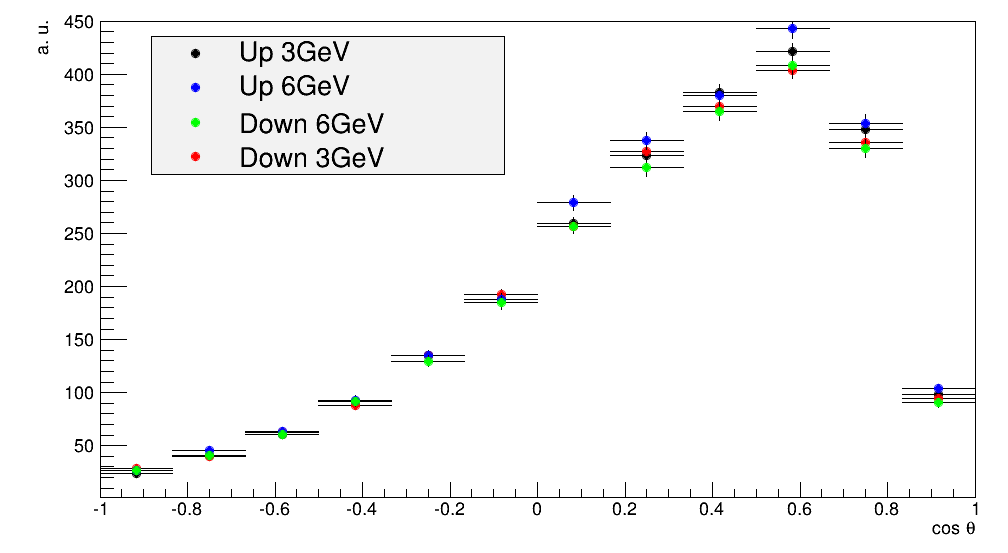
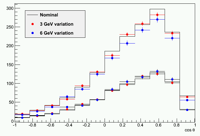
Table 3 :
     --> Why the new top mass uncertainties are so high ??? Even higher
that when considering the 6 GeV shift. I guess there is something wrong
here.

We do not have a clear answer. However the samples for up and down variation do show similar behavior to those of the 6 GeV samples leading us to conclude that it is indeed realistic that the uncertainty comes to the same value approximately (it was ~6% for mu and 4% for electrons before as well). As an example, find below the ratio plot of +- 3 GeV and +- 6 GeV to nominal:

Without the ratio:

And comparing individual channels of t_bar (down) and t (up):

In addition, we've performed a chi2 test between the various histograms:

	nominal	+3 GeV	-3 GeV	+6 GeV	-6 GeV
nominal	1.0	0.877789325027	0.609840681005	0.9998947065	0.990957296367
+3 GeV	0.877789325027	1.0	0.661343081089	0.845239939197	0.962327445115
-3 GeV	0.609840681005	0.661343081089	1.0	0.408133596257	0.968949641222
+6 GeV	0.9998947065	0.845239939197	0.408133596257	1.0	0.929692608053
-6 GeV	0.990957296367	0.962327445115	0.968949641222	0.929692608053	1.0

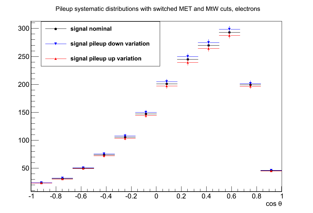
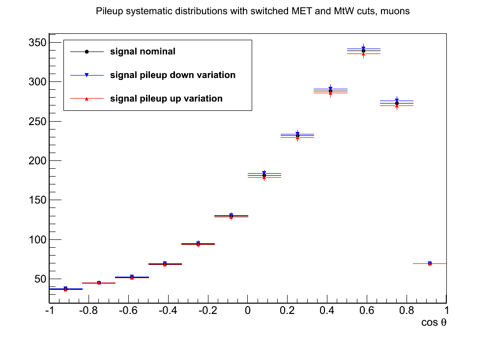
     --> Why the PU uncertainties are so much different between the
electron and the muon channels ?

Here again, the different behaviour of the MET and MtW cuts plays a role.

Here are the plots for muons and electrons with the standard cuts:

• 

• 

The discrepancy is larger for muons. However, if we switch the MET and MtW cuts for muons and electrons, this is what we get:

• 

• 

So it can be seen, that the difference in cuts is a reason for the difference in pileup uncertainty for muon and electron channels.

- Line 21-24 "However...", is that sentence really needed ? If you 
say that this is the first "precise" measurement of the top-quark 
polarization in the t-channel, that should probably enough ?

We would prefer to keep the sentence to illustrate the currently existing result.

- could you please add the cross sections that you used to 
scale the simulations ?

A table of MC cross-sections is given in Table 2 of AN and we are not sure, whether it is really needed to also show give this information in the PAS (that we need to keep in reasonable length).

 - just to make sure I understood, CompHep is a LO generator, so 
comparing CompHep with Powheg, you compares LO vs NLO ? If yes, you 
should say it in the text to justify the comparisons.

Yes and no: Comphep is LO, but these single-top t-channel samples apply a matching procedure based on the pt of the associated b quark (the one that is usually outside of acceptance) to mimic at least the bulk of the NLO behavior.
In the D0 papers (where they used Comphep with exactly this matching scheme as default generator) this was claimed to be "effective NLO", see page 5 here.
We now added this information, in the section about the MC samples, with a reference to the paper where this matching method was first documented.

 - Table 3 : the PDF and "sim stat." systematics are missing in the 
table. I'm wondering if they are really included in the total 
uncertainty of equations 6 and 7, because summing quadratically only 
what is in the table, I get exactly what is in the equations.

We have changed the description of "Simulation statistics":

"The uncertainty due to the limited amount of simulated events in the templates used for the statistical inferences (fluctuations in the background templates as well as in the elements of the migration matrix) are included in the statistical uncertainty returned by the unfolding method."

The statistics of the subtracted background samples are getting taken into account automatically by TUnfold and are included in the statistical uncertainty. We also include the uncertainty due to the limited amount of the events in the migration matrix and propagate the result through the error matrix to the statistical uncertainty of the asymmetry.

The uncertainty due to the PDFs is missing in the current version but we are working to incorporate that.

 - Line 92 : maybe add a reference for W and Z selection ? --> fix me

We are not sure that we are still synchronized with them. What about removing "from W or Z"?
Ideally one would like to cite some MUO and EGM POG documents, but unfortunately there are no public ones, up to our knowledge, that document these quality criteria.

 - Line 101 : "of around 0.1\% [...] true b-quarks, according to 
(which?) simulations". -- ???

Now we say "[...] true b-quarks in our signal simulation".

- Line 170 : Why Sherpa is used for the W+jets comparisons ? Could 
you justify and add the justifications in the text ?

We now changed the first paragraph of Section 5.2 by removing "which motivated a comparison with a sample produced with \SHERPA~\cite{Gleisberg:2008ta}" and adding:

"This discrepancy has also been observed in the comparison performed with data and simulation at 7~TeV in the context of a different analysis~\cite{Chatrchyan:2012ep}, and the investigation of different generators and of their settings shows that \SHERPA~\cite{Gleisberg:2008ta} provides a better description of \costheta\ in this control region at both centre-of-mass energies."

The reference Chatrchyan:2012ep is the t-channel cross section paper at 7 TeV.

 - Line 196 : "To decrease the model dependence", what does it means 
exactly ?

It is meant that the dependence on the MC simulation is reduced by fitting to data. The wording is misleading, however, and we have removed it from the text (as suggested also by Nicola)

- Lines 203-206, In the text, could you please better motivates the 
merging of shapes ?

In line 201 we explain that the criterion for merging is to have a fairly similar shape in both the BDT (the variable that we fit) and cosTheta (the variable that we unfold). Actually the similarity in BDT output is the most important, because if there is little discrimination, there is degeneration of the parameters from the fit. The similarity in cosTheta is way less crucial, although it is important at least that the main non-flat background (W+jets) is estimated separately from the main flat background (ttbar). But we are fine with the fact that, for example, s-channel (non flat) is merged with ttbar/tW/QCD (flat), as s-channel is so tiny that we can afford that. The shape difference of the template due to these minor background fractions is anyway taken into account as a systematic.

 - is Pt not dependent on the 4 parameters of equation ? Why to show 
Pt vs Vl and not vs the other parameters ?

In some models, Pt does depend on the others. But different models make this dependence different. The TOPFIT author insists on treating the top polarization as a free parameter because this ensures that the region allowed by the constraints covers all the possibilities without relying on model-dependent assumptions about the correlations.

We chose to show only Pt vs Vl because we didn't want to clutter the PAS with too many plots. The others may be proposed as supplementary material for approval, if you agree.
We are open to suggestions to which of the plots from the AN deserves to be also in the PAS.

- Table 4 : I guess the various parameters are treated independently 
to determine this table ? (because of interferences ?) It should be 
explained in the text and the caption. 

Yes. Done.

Editorial comments that are not listed are directly applied to the PAS

 - line 130: it is not clear how the values of the BDT cuts are chosen.
you mentioned that it is something related to getting the same efficiency 
of the cut based analysis for some specific working points but I think this 
has to be reviewed for the paper.

It is in our to-do list to optimize the working point based on the statistical and systematic uncertainties on the measured asymmetry. The preliminary checks have indicated that the currently used value is not far from the optimal value.

- line 174-181: this reweighing procedure for W+jets is not well convincing and justified.
a better understanding about the reason of difference spectrum in madgraph and sherpa 
is needed for further iteration. Do you have an idea of the reason of the residual discrepancy 
in the event yield ? is everything related to the statistic of the samples or something 
more fundamental ?

The madgraph-to-sherpa reweighting is only in shape and, by construction, cannot cure differences in yield. A similar difference in yield for the "W+light partons" component has been observed in cross-section analyses of the same process, motivating a data-driven extraction procedure.

- line 107:108: it is not clear why this cut at 0.025: is that so relevant? can you explain the 
rationale of that (light jet RMS cut)

The cut originates from the earlier t-channel cross-section analysis. The distribution is shown in AN fig 3 and the cut does improve the data-MC compatibility. However, we aim to optimize this selection for the paper.

- table 1: show that for W/Z+jets you have a factor almost two for the scale factor;
 is that understood ?

In the final event selection W+jets events contain a considerable heavy-flavor contribution that has been observed to induce the ~2 scale factor also in other analyses.

- I'm not fully convinced about the real utility of the combination 
of the electron and muon result for the asymmetry, especially because 
it seems counter-intuitive.

Indeed electron channel does not add much to the combination. However, since we decided to perform the analysis in both electron and muon channel, it still makes sense to also show their combination.

Section 6:
-- line 212-214: too technical. try to simplify if possible
Section 9:
-- line 327-332 seem too technical.

While they may be technical, they are short and provide relevant information. We would therefore prefer to keep them as they are.

    - rescale the top mass uncertainty assuming linearity (6->3 GeV),

Done.

    - for the W+jets uncertainty, perform the (QCD) fit with no constrains on 
the W+jets (instead of 200%) and see if the results changed. If it is 
stable, we could call it unconstrained in the text or better explain the 
justification for the 200% uncertainty.

The results are practically identical so we can just change the text. DONE

    - try to redo the BLUE combination but assuming no correlations for 
the QCD systematic,

Changing the QCD shape systematic from correlated to uncorrelated yields the same combined asymmetry within 2 significant digits.

scenario	mean	stddev
uncorrelated	0.4336	± 0.1236
correlated	0.4334	± 0.1237

    - after the reweighting of the W+jets sample (Madgraph vs Sherpa 
using the cos theta* distribution) check that other variables (in 
particular those related to the BDT) are not significantly changed,

We have checked how the following BDT input variables change upon applying the cos θ* dependent reweight. The input variables, and the BDT output as well, are very stable, with any variations being covered by already the statistical error of the templates. The results are summarised in the slides: https://twiki.cern.ch/twiki/pub/Main/PasTop13001QA/Sep3.pdf, slide numbers 3-9.

    - check the statistic in the t-channel sample with varied Q2 and 
verify that the larger systematics for the electron channel is due to a 
lack of statistics of the systematic samples,

The statistics for the systematic Q2 samples in the 2J1T MVA-enriched final selection is quite decent, with at least 3k events being available. However, doing this check we discovered that the anti-top scaleup sample was broken because of issues during crab -publish. We implemented an approximation where the anti-top scaleup shape is extrapolated from the top sample. Reprocessing the missing sample is ongoing as of last night and will be done in a few days, by approval by latest. The variated shapes, along with the statistics, are summarised in the slides: https://twiki.cern.ch/twiki/pub/Main/PasTop13001QA/Sep3.pdf, slide numbers 1-2.

    - check the plots (c) and (d) of Figure 1 and replace them with 
correct ones,

Done in PASv5.

Changes to be done on the PAS :

    - change the naming of "shape-independent" and "shape-changing" 
systematics,

DONE

    - clarify the text for the top pT reweighting systematic,

DONE

    - remove the "cut-based" column on the Table 1,

DONE

    - add systematics related to signal/background normalization in 
Table 1,

DONE

    - reduce the Section 7 (Unfolding) and rather refer to ttbar charge 
asymmetry paper,

DONE

    - for the limits calculation on anomalous coupling, please add 
explicitly that the input measurements are assumed to be uncorrelated in 
section 10, but also in the abstract and the conclusion. Say also 
explicitly in section 10 that it is a feature of TopFit.

DONE

Section 3:
Around L106: What motivates the difference in variable mT vs ETmiss for
the muon vs electron channel? I know it is too late to change this now,
but would also cutting on mT in the electron channel (but perhaps
tighter) work? Alternatively, why not cut on ETmiss for the muons? I
only ask since both channels are probing the same physics process, and
you have a fit template for QCD in the electron channel from an
anti-selected sample anyway...

This comes from studies made in the context of the t-channel single-top cross section analyses, since 2009.
The mT variable is a better discriminator against QCD in the muon channel, but not so good in the electron channel, where MET performs better. This is not so strange if one considers that "QCD", in the two channels, actually means very different processes: mostly bb and cc production with b/c->mu decay in the muon channel, while in the electron channel one has a cocktail where photon conversions and hadron misidentifications are very large fractions or even dominant.
You may also have a look at the answer given to the same question in 2009 (Cecilia's comments, section 3.8). Of course this has been re-checked by more modern cross-section analyses, like TOP-11-021, and we even rechecked ourselves in a very early stage of this analysis (but finding out the plots would require some skill in archeology...)

Around L107: I know that your selection is probably synchronised amongst
other top analyses but why do you use jets up to |eta|<4.5? Is there a
kinematic reason from the signal topology?

Actually here we differ from standard Top PAG analyses, where jets are typically considered up to |eta|<2.5 (where b-tagging is defined).
Our signal has a maximum around |eta|~3, as you can see in the |eta| plot in the AN (it's a feature similar to VBF production of the Higgs, and stems from the same kinematic reason: the jet recoils against a heavy resonance), and we stay away from the region |eta|>4.5 because it's at the boundary of the acceptance and anyway there are almost no events above 4.5.

Around L111: Why do you choose the TC algorithm and not e.g. CSVM? Also,
why is the Tight WP used? Would you not benefit more statistically from
the medium WP (improves efficiency by about factor 2 for mistag
0.1%-->1%) or does it just make things worse?

The reason is mostly historical: at a certain point the t-channel single top analyses were supposed to use the lepton+btag cross-trigger. This is based on TC, and therefore it was shown that using CSV offline gave awful turn-on curves, while TC had much nicer ones.
Of course this reason has became pointless in the meantime, because we chose to make our life easy by using only single-lepton triggers (although in the future we may reconsider the cross triggers to lower the lepton threshold).
A reason for not changing (or at least for decreasing the interest of changing) is that in our signal region the W+jets process is by far dominated by W+c (followed by W+cc and W+bb), and W+light is only a negligible component. The CSV algorithm does not improve the discrimination against c quarks as spectacularly as the one against light partons (intuitive reasons: also c quarks produce secondary vertices, and CSV relies on them).
And we chose the tight working point, as all t-channel single-top analyses do, because with the medium working point the W+jets category would blow up, and it is the background that we fear the most, being in general quite poorly modeled in this region of phase space (for our needs at least). You can see how much pain we took to model cosTheta properly for W+jets, in the AN.

Around L117: How is this cut motivated? It seems like 0.025 is 50% of
the cone size. In principle you could also apply this to the b-tagged
jets, but I suppose you trust these jets as they have passed the b-tagger?

We borrowed this cut from TOP-12-011 (cross section at 8 TeV), where it was optimized "by eye" against pileup jets. Details can be found in the companion AN of that PAS. (The corresponding paper, which is now starting review, has a different Cadi number, TOP-12-038, because it was merged with another analysis. But it still uses the same cut.)
At that time it was seen that it was not advantageous to apply it to b-tagged jets. This is understood, by considering that b-tagging itself is an implicit guarantee of quality of the jet (it implies that at least some high-quality tracks are associated with the jet.)

Around L121: Do you take into the signal contamination? i.e. the signal
(and background) is not exclusive to one bin.

Yes, for example in 2j0t, that we use to improve the W+jets modeling, we subtract the signal contamination as well as all non-W backgrounds. Of course in principle this induces a circular logic, but the signal component is very tiny, as can be seen in the plots.
The other control regions, 3j1t and 3j2t, are only used for qualitative validation of the ttbar model, and not to extract templates or other active uses, and therefore no signal subtraction is needed there.

Around L126: Does this also apply to the 0tag categories i.e. you simply
use the discriminator value even if it's not b-tagged?

Yes, whenever there is an ambiguity on which jet should be used to build the "top candidate" (which is quite an artificial concept in 2j0t, but we need it to define some of our variables), like in 2j0t, we take the jet with largest discriminator value. Although this is essentially like taking it randomly, whenever the process has no real heavy flavour (Wgg, Wqq, Wqg) or has two (Wbb, Wcc). In 2j0t, processes with just one heavy flavour (like WcX) are not dominant.

Around L142: How do you justify the BDT discriminator cuts i.e. 0.06 vs
0.13? Is there some working-point chosen e.g. X% purity based on Fig.1?

Purely historical reasons: until a couple of weeks before preapproval, we had no BDT, and we had a cut-based analysis, then fitted |eta| of the untagged jet.
These cuts just give the same signal efficiency as the old cut-based analysis.
We planned to perform an optimization of this threshold very soon, but given the very tight deadline for green light, probably we will stick to these thresholds... Anyway, for the final paper we would like to have optimal thresholds.

Around L145 and Table 1: I am a bit confused about the bottom-line here.
How do you justify the cut-based quantities versus the BDT i.e. why
choose |eta of non-tagged jet| > 2.5 and 130 < m < 220? Can you quantify
the differences between the cut-based and BDT, and also the electron and
muon channel? I understand that you want to show a "sanity" cross-check
but I think it is missing a few details.

Actually it may make sense, now, to remove any reference to the cut-based analysis, as it doesn't really bring new information. It made sense to keep the side-by-side comparison, when we first introduced the BDT approach, because the very first readers of our PAS were more familiar with the cut-based and naturally wanted to compare to that. But now, maintaining two analyses in parallel is quite an extra burden, and not so motivated.
Those two thresholds are, again, just historical: the top-mass window was optimized in the context of the cross-section analyses (TOP-11-021 at 7 TeV, TOP-12-011 at 8 TeV) and the |eta_j'| cut also comes from there: in those analyses, as a cross-check of the validity of the measured cross section, it was shown that cosTheta (defined exactly as we do) had a good data-MC agreement, when the fit results were used, in a region enriched in signal. To enrich in signal, this |eta_j'|>2.5 cut had been chosen "by eye" (no serious optimization was deemed important, as the only point of this cut was to make this cross check, and it was not really used to get the cross section.)
About the quantification of the differences, you can find in the AN the results of the fit, in both channel, with the cut-based approach and the fit of the |eta_j'| variable. Results are consistent with the BDT fit.

Section 5:
Around L167: I had to read it several times to understand that you fit
mT for the muon channel and ETmiss for the electron channel. However,
why do you constrain the W+Jets to +/-200% of the expected yield? This
seems excessive, especially given you use the NNLO x-sections (I am
assuming you only float the normalisation?) Also, what are the ranges
used for each of the fits (in mT and ETmiss)? Is there a sensitivity to
the ranges used?

The large uncertainty is due to poor MC modeling of W+Jets. In the QCD fit we also use shape uncertainties of JES, JER and Unclustered Energy in addition to the normalisation. The ranges for both muons and electrons are from 0 to 200 GeV. AN Tables 5 (for muons) and 6 (for electrons) show the results with different fit ranges (and anti-isolated regions). The fit is not sensitive to the ranges used.

Around L183: Are you sure there is no circular argument here given that
you have already used a W+Jets fit in the QCD background estimate?

In this paragraph we don't refer to the discrepancy in yield (that is also present, see below), but in cosTheta shape.
And the QCD yield estimation is based on variables with relatively mild correlation with cosTheta.
Circularity is more of a conceptual issue for the step described in l.197-199: in that case, we attribute the discrepancy in yield to a component of W+jets (so, if we misestimated QCD, we misestimate this one too). But this component turns out to be very negligible in the signal region, and even a 100% uncertainty on this correction gives no visible effect.

Around L189: It was not clear which generator makes the approximation of
the massless quarks.

Sherpa. (In our official CMS sample, of course, and not in general: Sherpa is perfectly able to deal with that, if all diagrams are explicitely generated, but this particular sample had been probably requested in the context of W+Njets analyses where b-tagging was not applied or not important.)
You are right that the text is ambiguous; we are changing "of this sample" into "of the latter sample".

Figures 2-4: The ranges of the ratio plots are not consistent. Also
there is no * on the cos(theta) axis label.

Fixed in PASv5.

Section 6:
Table 2: The fit for the signal appears inconsistent between the muon
and electron channels. I would naively have expected that they should
agree. The only key difference I can think of (other than the treatment
of QCD) is the ETmiss vs mT cut which probably changes the sensitivity
of the procedure. Is it possible to test this hypothesis by performing
an ETmiss cut in the muon channel (or vice versa). Or rather, have you
tested that this difference does not introduce a bias in any way?

Here are the fit results for both muons and electrons with the different cuts:

Muons with mT cut:

• signal: 0.98 +- 0.03
• Top + QCD: 0.84 +- 0.06
• W/Z+jets 1.88 +- 0.13

Electrons with mt cut:

• signal: 0.93 +- 0.04
• Top + QCD: 0.80 +- 0.08
• W/Z+jets: 2.23 +- 0.18

Muons wth ETmiss cut:

• signal: 0.90 +- 0.03
• Top+QCD: 0.83 +- 0.06
• W/Z+jets: 1.99 +- 0.17

Electrons with ETmiss cut:

• signal: 0.88 +- 0.04
• Top + QCD: 0.89 +- 0.07
• W/Z+jets: 1.97 +- 0.20

So we can see that indeed the difference here comes from using ETmiss vs mT cuts in different channels.

Section 7:
Arounds L239 and L246: some repetition, needs merging?

Thanks for spotting, we have merged these paragraphs.

Section 8:
Around L314: This paragraph confused me and should probably come before
the description of the various systematic sources. Can you explain what
you mean by it? Also, do you assume each uncertainty is symmetric in the
upward and downward variations? Have you checked this?

This paragraph was left over from the old method. The now used data driven method is explained in the beginning of this section.

We don't assume each uncertainty is symmetric, we check the up- and downward variation and take the maximum of both to be conservative. The quadratically added sum of up- and downward variations is very similar to each other and the sum of the maximum uncertainties.

Section 9:
Around L327: There is some degree of correlation between the overall
systematics, but the statistical uncertainties should be uncorrelated
(by definition of the selection). In this case, can you not put some
sort of a significance on the difference between the electron and muon
results?

Considering all the uncorrelated uncertainties (statistical + some of the systematics), the difference is at the level of 0.9 sigma. Do you advice to mention that in the PAS?

Also, when it comes to the combination, technically speaking, could you
not have repeated the procedure but fit both the electron and muon
channels simultaneously? While Ref[40] is an interesting read, it would
be good to simply do the combined fit and compare to this result. It
looks as though the electron channel does not add so much to the final
measurement which makes me a little uneasy...

We decided to combine at A_l level, because fitting the electron+muon sum requires some technical gymnastics in order to deal with the different unfolding matrix of the two channels (selection efficiencies are different, backgrounds are different, and in principle also the resolution part of the matrix is different). In principle the result should be the same in the end, although we didn't check.
Concerning the electron channel, indeed it is rather useless in the combination, but this was expected (higher thresholds, lower purity). In an early stage of the analysis we were even planning to only use the muon channel, but then we felt that it was important to have the second channel to cross-check the main one and to avoid giving the impression that we were hiding something under the rug.

    - I think that the "\int L dt" in the plots text could be replaced 
with a capital L, and the text in the TPad could be then increased

OK.

    - given the uncertainty on the luminosity, I would use L=19.7 or 
maybe een L=20 fb^{-1}, instead of 19.75 nd 19.72.

OK.

    - in the ratio plots (exp-meas.)/meas., I would use the same range 
for the y-axis for all plots (this makes comparisons easier), [-1,1} 
should be ok for all plots.

Sure, but in some cases, as you mentioned yourself, the variations are much smaller than 100%, so [-1, 1] would make discrepancies invisible. Which would then be preferred?

    - what "all syst." means in the TPad ?

It means that all systematics are included (as opposed to, for example, only JES). It was included for debugging and is indeed spurious in the PAS, so it will be removed.

    - the size of the legends could still be increase. I still found 
them a bit difficult to read.

Agreed.

Figure 1 : the systematics are missing for plots (c) and (d). The 
caption is partially outside the page, so I can not read it completely.

It will be added very soon, it was missed in a rush (also fixing the cosmetics).

Table 1 : I think you said the caption was not updated ? While there is 
a nice agreement for the electron channel, for the muon channel the MC 
prediction is still 2 sigma below the data. Are the uncertainties on the 
background normalization accounted in the errors ? Uncertainties on the 
signal normalization ? If not, it might be good to include them, to show 
that actually the data and MC yields are compatible within the 
uncertainties.

The uncertainties are only MC statistics at the moment, which do not reflect the true uncertainty. It is on the TODO list to update this table to the recipe you suggested as soon as possible.

Figures 2, 3 a,d 4 : in the ratio plots (exp-meas.)/meas., the 
uncertainty bands are out of range.

Sorry. We will fix this.

Equation (8) : the combined value is higher (0.43) than the 2 individual 
measurements (0.42 and 0.28). This suggest that one of the two 
measurement as a "negative weights", meaning a negative contributions to 
the combination. This is usually happening when one single measurement 
as a much larger uncertainty than the others, and which has a strong 
correlation. Thus, I'm expecting that the electron channel has a 
negative weights. Could you check that ?

Yes, that's the reason, the muon channel has a weight of 110%, the electron channel of -10%.
You can see that the AN is now citing the recent study by A.Valassi and R.Chierici that explains very nicely under which conditions this happens. As you noticed, we are exactly in those conditions: the electron channel has larger correlated systematics. It was not happening before, because we were over-estimating the MC-stat systematic (which is uncorrelated), so the electron weight was small but positive.

I think that some of the backgrounds uncertainties could be treated as 
uncorrelated among the two measurements. In particular, the QCD shapes 
are taken from data in statistically uncorrelated samples. That is 
probably too late to consider this, but keep it in mind for the paper.

Probably we can consider it in time.

Table 3 : I have the same comment that Oliver. There are large 
differences between the electron and muon channels. The JER is a good 
example, because I would have expected it to be small for both channels. 
Also, the uncertainties changed quite significantly (decreased) with 
respect to v3. Could you explain why ?

See the answer to Oliver's question below.

Figure 5 : the legend is still a bit small. I see that the error bars 
are much smaller in v4 than in v3, why ? The shape is also quite 
different for the electron channel, could you explain the modifications 
to the analysis which explain such differences ?

Cosmetics will be improved.
The main reason for the shrinking of the error bars is that in the previous drafts we were badly overestimating the MC statistics systematics, due to some bug.
Please notice that we also changed the binning, with respect to v3, and this gives the false impression that the error bars shrank more than they did, and that the shape in the electron channel changed (in reality it didn't: if you compare the old and new pictures side by side, you can see that the excess and the deficit are in the same place as before).

Table 4, Figure 6 and 7 : The g_L/R and V_L/R parameters are I think 
parameters of the effective lagrangien. For the reader to understand, it 
might help to have the expression of the Lagrangien written somewhere in 
the text ? Maybe after line 333 ?

Now added.

- line 32-33: do you mean the measurement of top quark polarization in
single top events?

Yes. Thanks for spotting that, now it's corrected.

- BDT: The signal-to-background ratio is definitely improved with the BDT,
especially for the electron channel. Should we quantify the improvement in
the text?

We think that it would not be necessary, as the plots of Figure 1 are quite self-explanatory, but if the ARC thinks that it can be informative, why not.

- Unfolding: I had a quick look at the AN concerning the unfolding, and
would be interested to look at the linearity test. I don't understand
though how you are going to show the linearity with the prescribed
procedure. I would vary the polarization by reweighting and compare the
true polarization with the unfolded result? I expect the linear fits to be
very good, but small deviations could be used as systematic error.

This is now added, and the text will be expanded in the next AN draft, hoping to make it more clear.
The procedure to test the linearity of the method is as exactly as you describe it in your comment. We vary the true polarization by reweighting the events and compare the result we get from the unfolded distribution with the true polarization. For each different polarization pseudo experiments are performed and the mean value of the measured polarizations is compared to the true value. The following figures are for the very same setup as in the PAS draft v4 (we specify that, because the BDT cut will change in the next draft, and the linearity tests will be updated):

• Muon channel:
  

• Electron channel:
  

As can be seen, the linearity is very good but there is a small bias. This bias is negligible with respect to the statistical error of the single measurement and to the main systematics.
We will quote it as an additional systematics.

- Systematic errors: Do you know why the systematics for electron events
are so much larger than for muon events? Maybe this is a naive question,
but the JER is 0.005 for muons and 0.134 for electrons.

For the difference in JER, the reason seems to be different MT/MET cuts in the channels. Looking at the discrepancies between JER up and down variations, the difference seems larger close to the maximum of the distribution, where MT/MET defines the behaviour.

• JER up and down variation comparison for muons:
  

• JER up and down variation comparison for electrons:
  

By changing the cuts for muon and electrons - applying the MET cut on muons and the MT cut on electrons, we get the following distributions where the discrepancy is now larger for muons.

• JER up and down variation comparison for muons: with MET>45 GeV cut instead of MT>50 GeV
  

• JER up and down variation comparison for electrons: with MT>50 GeV cut instead of MET>45 GeV
  

So we can conclude that this is the cause of the difference for JER.

- top mass systematic: What are the variations from nominal, and what was
nominal (apologies, I didn't read the AN)?

The up and down variated templates are produced using samples where M_top = 166.5 / 178.5 GeV at generation, the nominal is 172.5 GeV. This is applied for the ttbar and signal samples.

- top pt reweighting: for 7 TeV dileptons, we were asked to show the top pt
reweighting separately from the other systematics. The systematic error is
small in this case, but we should check with the convenors if we should do
the same here. I think you don't apply the correction to the measurement
and only quote a systematic error (I might have missed that while reading)?

We actually apply the correction as one of the updates in this latest round, and also apply a systematic variation on this reweighting as per the recipe [1] (up=weight^2, down=weight^0, nominal=weight^1, where weight is given as a polynomial function of the top pt at gen-level). Applying the top pt correction makes the pt spectrum softer and have a better agreement with data in the 3j2t ttbar-enriched region as can be seen on the following plot.

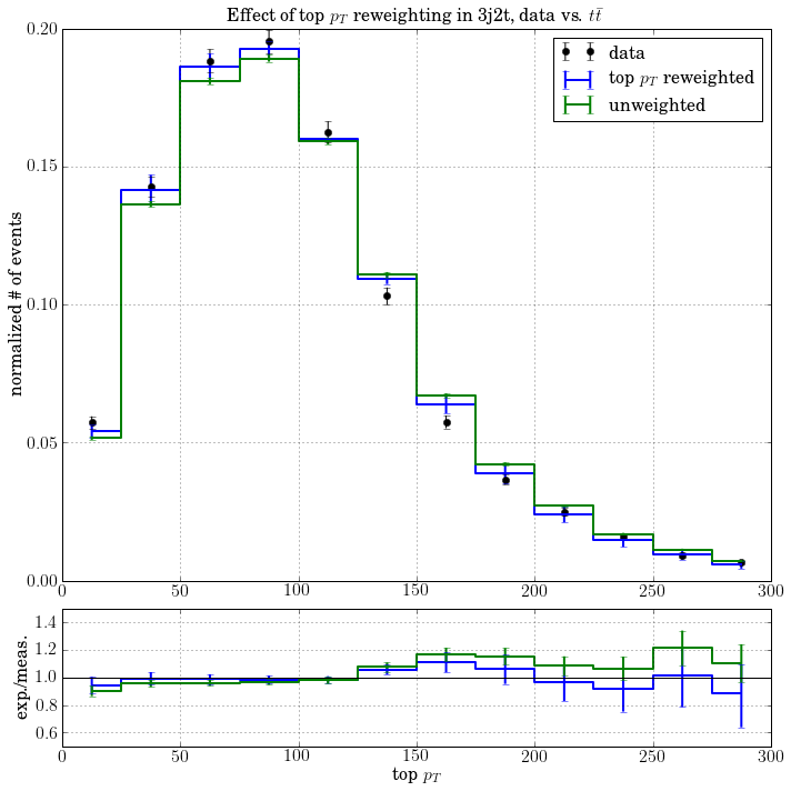The effect in cosTheta is much more mild, which iseven smaller in the 2j1t signal-enriched region having a lower ttbar contamination.

In the 2J1T region after applying the MVA cut, any shape differences between the weighted and unweighted distributions from ttbar are negligible.

[1] https://twiki.cern.ch/twiki/bin/viewauth/CMS/TopPtReweighting

Jeremy's reply:

Just to make sure I understand, the difference between 2) and 2') is that,
 in 2) the QCD normalization is floating (as part of a merged template) but
 has a fixed fraction within the template, while for 2') the QCD normalization
 is really fixed and not allowed to change.

Your understanding is correct.

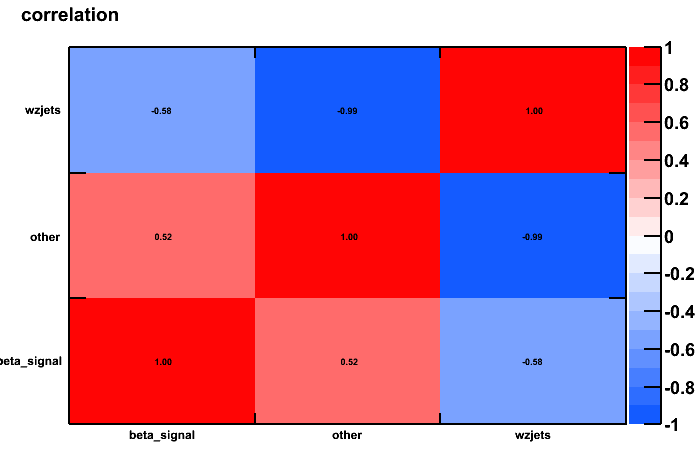
How difficult would it be to switch to the new approach and how much would it
 change the results? Even if the two approaches are different, they should
 give compatible results within the uncertainties. Could you check that easily ?

We tried, and here is what we get:

The new fit results are (scale factor +- uncertainty, qcd sf is by definition 1):

muon: beta_signal 0.95 +- 0.05 other 0.77 +- 0.10 wzjets 2.02 +- 0.22

electron: beta_signal 0.85 +- 0.06 other 0.85 +- 0.11 wzjets 2.10 +- 0.32

To be compared to the old ones in Table 2 of PAS v4 Sep7.

The new correlation matrix for the muon channel is:

electron channel

To be compared with Figure 46 of AN v7.

Propagating all the way down to the end of the analysis, we now get A_l = 0.46 (muon) and A_l = 0.304 (electron).

The QCD rate systematic is now 0.24/0.07 (muon/electron channel), the QCD shape systematic is now 0.014/0.05.

Conclusion: FIXME

 The main important points are :

     - binning/axis ranges should be adjusted for some plots,

I have adjusted the visual style of the plots on figure 1, figures 2-4 will receive the same treatment.

     - Table 1 should includes the data-driven normalization, as well as
all the plots.

This was now taken into account, thanks for pointing it out.

Note: just realized that we forgot to update the caption of Table 1 accordingly, and the uncertainties in that table are still from MC. To be fixed in next draft.

     - errors in the plots should probably include the uncertainties on
the normalizations and (if it is possible) the main systematic sources.
This would help to demonstrate that the remaining data/MC discrepancies
are well covered by the systematics.

The systematic error band evaluation is now an option and the main data vs. MC plots display the shape uncertainty resulting from the various systematics.

Abstract : I would removed "under the assumption that the spin analyzing
power of charged leptons is 100%", 100% is a very fair and usually value ?

We would like to make a difference between the first P_t value that we quote, which is just A_l times 2 (i.e., it assumes the SM value alpha_l=1), and the one that we quote at the end, which comes from TopFit and doesn't assume alpha_l=1, as the latter is modified by anomalous couplings.
An alternative could be to present the first number as the measured P_t "under the SM assumption", but this would bring the logical contradiction that if we assume the SM then we also have a prediction for P_t and we don't need to measure it.

"Combining the measured [..] CMS measurements ", I suggest : "Combining
the presented asymmetries with the CMS..." to avoid repetition of "measr.".

OK

"without a prior of the assumptions on the spin analyzing power of decay
products" is it true ? You just say you take 100% for charged leptons. I
suggest to clarify or simply to remove that part of the sentence.

Here we want to convey the message that, differently from the P_t value that we quoted just before, now we are going to quote a P_t value where we don't assume alpha=1.
We are open to suggestions on how to make it more clear.

     - "limits are set on the Wtb anomalous [...] obtaining Pt> X at
95%", naively, I would have expected that the quoted limits would be on
the parameters of the effective lagrangian in equation 23 of the AN. So
I'm not sure what the limits on the Pt means? Is Pt not dependent on the
parameters in eq 23 ? Could you tell me how I should understand this
limit and how it translates into limits on the parameters of the
effective lagrangian ?

The effective extension modifies the coupling structure at the Wtb-vertex. So if one knows the top quark spin orientation (meaning its chirality at the vertices), one can calculate the asymmetry directly from the anomalous couplings. However, the top quark spin is assumed to be "only often" in the direction of the spectator quark. The polarization quotes therefore the spin alignment of the top quark with the spectator quark.

The fact that only known vertices (and their couplings) are present in the SM t-channel single top production enables theorists to calculate the polarization for the SM case and even for the effective Wtb coupling case in terms of the anomalous couplings. This has not yet been done but its is in principle possible to calculate Pt=Pt(VL,VR,gL,gR).

Nevertheless, the anomalous couplings stem from an operator product expansion. This ansatz does not account for a possible more exotic top quark production mechanism like 4-fermion interactions. Therefore, we keep the polarization independent of the anomalous couplings by assuming a flat prior.

More information are given in: J. A. Aguilar-Saavedra, et. al., W polarisation beyond helicity fractions in top quark decays, 2010 http://arxiv.org/abs/1005.5382 In the footnote on page 24 it is said: "One could still argue that the single top polarisation is calculable in terms of the Wtb couplings. However, this assumes that no other new physics, e.g. four-fermion operators, contributes to t-channel production, and turns the results model-dependent."

     - bullet on line 33 : is there an explanation for the issue on the
eta_j distribution ?

This region seems to be covered in 2J1T by the systematic errors.

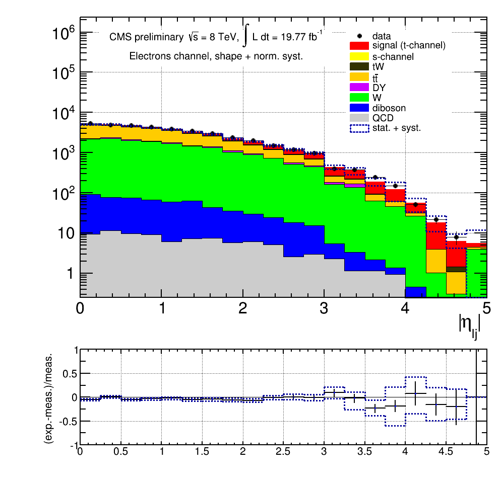In 2J0T, without applying the signal-enriching MVA and allowing for both shape and normalization systematics, there seem to be hints of a mis-modeling at very high η (>4.5), with higher statistics in MC a more careful study should be conducted.

Similarly, there seems to be an effect in the unenriched 3J1T sample which is not covered by the present systematics.

Low statistics in both data and MC do not allow conclusions to be drawn there at the moment.

     - line 55 replace "which" with "and" ?

OK

     - line 58 "single-top quark"

Changed into "singly-produced top quark"

     - line 58 ; I suggest rephrasing " the precision was not sufficient
to reach a conclusion on the top-quark polarization"  or something similar ?

We propose:

"the precision was not sufficient to reach a conclusion about the sign of the polarization of singly-produced top quarks have the opposite polarization."

     - after line 59 : " the top-quark-spin asymmetry" ?

OK

     - line 60: I found it a bit difficult to read, here is a (probably
imperfect) proposal of rephrasing : "The spin-analyzing power $\alpha_X$
is the degree of correlation between the spin of a top-quark and the
angular distributions of its decay products. In the SM, it is exacly 1
for charged leptons".

OK

     - line 63 : "top-quark couplings"

OK

     - line 64 : "top-quark polarization"

OK

     - line 65 : "top-quark spin"

OK

     - line 65 : "single-top quark"

Not sure about this... Here "single" qualifies "top quark" and not just "top".

     - line 67 : "top-quark polarization"

OK

     - line 68 : "decay channels. It is based on an integrated
luminosity of 19.8 fb^{-1} of $\sqrt{s}$ 8 TeV proton-proton collisions,
recored by the CMS detector [3]." or something similar.

OK

     - line 73 : "top-quark polarization"

OK

     - line 74 : "top-quark-spin asymmetry"

OK

     - line 77 : "top-quark couplings"

OK

     - line 88 : "Z+jets" => "$Z/\gamma^*$+jets".

Now changed everywhere in the text.

     - line 88 : Could you also specify the number of additional partons
? Especially for W+jets and DY.

Added:

"Up to three (four) additional partons are generated at matrix-element level in \ttbar\ (\wjets\ and \zjets) events."

     - line 95 : "with pythia events ..." what does it means exactly ?
That you use QCD pythia events to check the data-extraction of the
multijets ? BTW, I would use the term "multi-jets" rather than QCD
everywhere in the text.

Your understanding is correct (although the check is of very limited use in practice, given the poor MC statistics after the cuts).

We added
"(henceforth indicated as ``QCD'')"
the first time that we introduce the term.

     - line 97 " top-quark mass"

OK

     - line 99 : "single-top processes"

OK

     - line 107 : "number of observed primary vertices between data and
simulation" => That plot is missing in the AN

Now it is shown in section 7.10 and figure 53 in the AN.

     - line 111 : "one isolated charged lepton and a significant missing
transverse energy". ",MET," => "(MET)",

OK

     - line 112 : " W-boson decay, as well as ", " top-quark decay"

OK

     - line 113 : "additional light-quark jet from hard scattering
process, which is preferably produced in the forward region"

OK

     - line 116 : "Electrons or additional muons ...", I think this
sentence is outdated, and should probably removed anyway. I would rather
add it after the presentation of the lepton selection.

You are right, this information is anyway given at the end of the lepton selection paragraph.

     - line 117 : "The trigger providing the data sample", "The trigger
selection is based ..."

OK

     - line 123 : "are removed from the particle list" => "are vetoed"

OK

     - line 126 : "passing quality and identification criteria" and
remove the parenthesis in line 127.

OK

     - line 129 : "looser quality, identification and isolation criteria"

OK

     - after line 129 : I would remove the "," in "contamination, in the
electron" and instead add one here : "electron channel, a threshold..."

OK

     - "with m$_T$ defined as "

OK

     - line 130 : replace "defined" by "reconstructed" to avoid
repetition with above equ (2)

OK

     - lines 134 to 139, I think the few sentences could be shorter. No
need to give details on the b-tagging algorithm itself. I would just say
: "In order to [...] b-tagging algorithm [23] with tight selection on
the b-tagging discriminant, which corresponds to light-jet mis-tagging
rate of 0.1\%, as estimated from simulated multi_jet events". It could
be also interesting to quote the b-tagging efficiency for signal events.

We shortened the text as you suggest, but maybe better not to give detailed numbers (which depend on pt, eta, etc. anyway), so what about:

" which corresponds to a light-jet mis-tagging rate of around 0.1\% and an efficiency of around 40\% for jets originating from true b quarks."

     - line 140 : "for true and fake b-jet" => "for light and heavy
flavor jets"

OK

     - line 145 : "is required" ?

OK

     - line 150 : "as discussed in Section 5", to stay consistent in the
way you refer to other sections ?

OK

     - line 158 : " The C-parameter, defined as ...". Is it really a
"parameter" ? Should it be rather called "C-variable" ?

We found that this is the usual name in the HEP literature, see for example:

http://arxiv.org/abs/hep-ph/9801350

http://arxiv.org/abs/hep-ph/0306094

http://cds.cern.ch/record/386138/files/9904033.pdf

     - line 168 : I would replace "A threshold of .." with something
like, "To further enriched the sample in signal, events in the muon
(electron) channel with a BDT output smaller than 0.06 (0.09) are
rejected".

OK

     - line 171 : "threshold" => "selection", if I'm not mistaken,
threshold usually refers to energy/momentum selection, especially at
trigger level ?

We have seen other examples of this use of "threshold" in published papers.

     - same line : "is replaced by the following requirements : ..."

OK

     - I have a fundamental problem with the Table1. I think it should
not be shown has it is. The data/MC agreement of the yields are quite
bad, especially for the muon channels. This give the impression that you
perform your measurement with large data/MC disagreements. But the
numbers in that table are not the ones you are using for the analysis !
Things should be much better after accounting from the signal/background
normalization "scaling-factors", determined from data. So I would
strongly suggest to include these SF in the table, and possible move the
tables (and all the plots) after the discussion on backgrounds in
sections 5/6.

The contents of these tables have been changed to reflect the results of the fit on the BDT output variable.

     - Figure 1 : here are some cosmetics corrections (those are
important plots, so I'll be picky ;) ),
         * could you try to increase the size of the legend where it is
possible ?
         * replace "BDT" with "BDT output" for the label of the x-axis ?
         * In the error bars, I would include the uncertainty on the
data-driven normalizations, it should show that the 10% excess of events
in data is well covered by these uncertainties.
         * If this is technically possible, it might be good to add also
the uncertainties on the shapes. I understand this is usually
complicated to do, so please tell me if you don't think this is possible
in a decent amount of time. But this would help to check if the "bump"
in data around -0.4 for the cos theta distribution in the electron
channel is covered by the shape uncertainties.
         * Top plots : could you enlarged the y-axis range of the ratio
plot ?
         * Middle plots : I would also enlarged the y-axis range of the
ratio plot, and try to find a better binning, there is quite a lot of
statistical fluctuations.
         * Bottom plots, same corrections as Top and Middle plots.
Clearly the legend could be larger.

Thanks for these useful suggestions. We've made the cosmetic changes and introduced the shape uncertainty band. At the moment, the normalization uncertainty is not shown (TODO).
In the mean time, we see that already including the normalization uncertainty from other sources (without additionally taking into account the uncertainties scale factors form the fit), any discrepancies are covered. This is by far dominated the uncertainty of 100% on the W+jets yield.

     - line 180 : "where \Gamma is the decay width of the top quark, P_t
the single-top ..."

OK

     - line 182-183 : this is somehow a repetition of what is said in
the introduction.

OK

     - line 187 : "top-quark rest-frame" ?

OK

     - line 201 : "also loosening the electron identification".

OK

     - I have another question on the analysis, which shows-up only now,
while I'm reading the background section. The QCD background is
determined from mT and MET, but these 2 variables are used in the BDT
training, so there are also used through the BDT to estimate the
normalization of other processes (which are free in the BDT fit). So I'm
wondering if there are some correlations between the 2 fits, which could
leads to some underestimation of the total uncertainty on the fit ?

The result of the MET/mT fit for the estimation of the QCD yield is driven by lower values of MET/mT that contain majority of the QCD contribution and that is cut before the mva is trained. Thus we expect the correlations between the fits to be negligible. Note that the QCD yield that is obtained in the full MET/mT range is well compatible with the yield that is obtained in the MET/mT region below the preselection threshold (see table 5 and 6 in AN v5).

     - line 205 "(see in Section 8)" => ", "discussed in Section 8",

OK

     - line 221 :" verified at generator level", remove the "private"
stuffs.

OK

     - line 222 : I would rephrased a bit : "In addition, the
application of the re-weighting conducts to a residual discrepancy in
the event yield of 11\% (???). It has been [...], and therefore this
component is rescaled accordingly in the signal and control regions." Or
something similar.

OK, rephrased in a similar way to what you suggest.

     - Figure 2, (a) and (b) : this time, probably the y-axis of the
ratio plot should be smaller ;), especially for (b). The ratios plots of
(c) and (d) shows increasing points at -1 and 1. Is it covered by
systematics ? It would be good to demonstrate it in the plot. Did you
include the data-driven normalizations ? If not, I would introduce them,
as well as the corresponding uncertainties.

These useful suggestions have been taken into account in PAS v4. Any discrepancies are covered by the yield uncertainty of W+jets. The data-driven normalizations were not taken into account, since strictly speaking they were derived in a different phase space (2J1T), and the relatively large anti-correlations between W+jets and the other background categories suggest that dramatically changing the W+jets yield from 2J1T -> 2J0T would also change the scale factors.

     - Figure 3 : adjust the y-axis of the ratio plots. Did you include
the data-driven normalizations ?     If not, I would introduce them, as
well as the corresponding uncertainties.

PASv4 now shows these plots with the systematic uncertainties (shape and yield). The uncertainties on the data-driven scale normalizations were not taken into account yet, which will be done in the table 1 of the PAS.

     - line 257 : "After subtracting the background, a regularized..."
The background subtraction is discussed on line 261.

Swapped order, and removed "with the procedure of the preceding section"

     - line 283 : a space is missing after "correctly. A ..."

OK

     - line 286 : "top-spin asymmetry"

OK

     - line 289 : it could be good to described in few sentences how
this is done. That is not obvious, at least to me.

The method to estimate the systematic uncertainties has changed. We now repeat the measurement on data using the shifted systematic templates for the BG-fit and the unfolding procedure (as for example done in the ttbar charge asymmetry measurement). Thus, the sentence in line 289 has been replaced with a short paragraph describing the method.

     - line 290 : the lepton selection efficiencies could very well
affect the shape of the cos theta* distribution. In particular, the
isolation requirement could have a non-negligible effect (it has in the
ttbar W helicity measurement).

True, isolation is expected to have an effect on the high-end of the cosθ distribution. We didn't consider that so far, as it is difficult to justify that it is independent from other systematics. We see that in TOP-11-020 (W-helicity measurement in ttbar) a shape systematic is considered, in the muon channel, by comparing the eta-dependent lepton scale factors with a flat scale factor (a more complex procedure is applied in the electron channel, where they apply a complex procedure based on shifting the electron-leg and jet-leg scale factors of the e+jets cross trigger such to maximize the eta effect; we cannot do the same, as we use a single-electron trigger.)

We have considered the idea to follow the same method as TOP-11-020, but we believe that this would not have the desired effect (and possibly no visible effect at all).

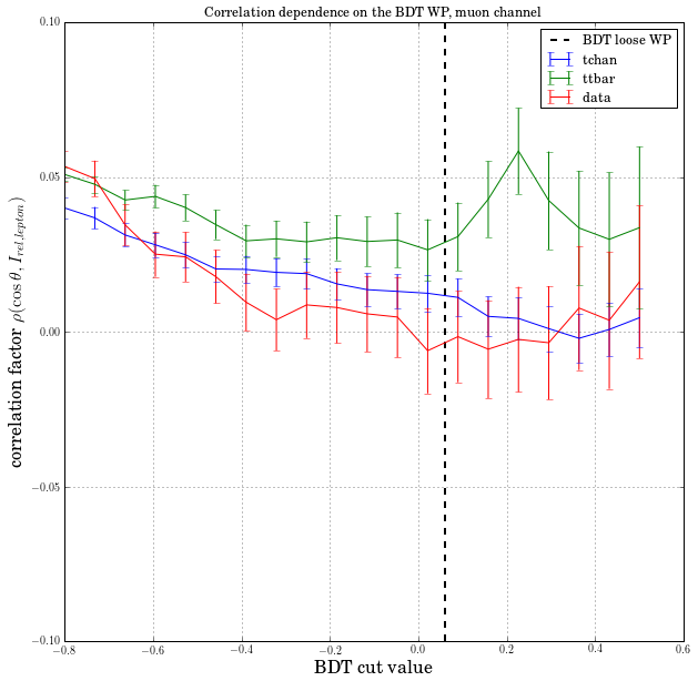
There is, indeed, a correlation between the lepton eta and our variable of interest, that depends on the BDT cut as you can see here:

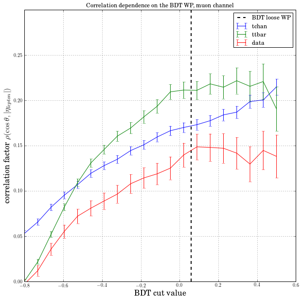Nevertheless, variating the lepton-eta shape as in TOP-11-020 doesn't seem to give a visible effect:

• JA : did you check the pT dependence ? Is it expected to be negligible ? Are the plots made after or before the BDT cut ? I guess this is signal only ?

We checked the lepton pt cut dependence on the correlation(cos θ, lepton η) and it is indeed negligible, with a slight tendency to decrease at harder pt cut values.

We have also checked the effect of the POG-provided lepton eta-dependent weight on the cos theta shape, by varying the weight around unity. There is a ~2% shape effect of this variation on the variable of interest, which will be taken into account as an additional systematic. These studies are summarised in https://twiki.cern.ch/twiki/pub/Main/PasTop13001QA/Sep2.pdf.

Additionally, we've evaluated the correlation with respect to the isolation variable, which is <5% in all cases.

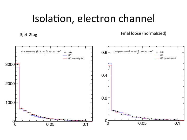
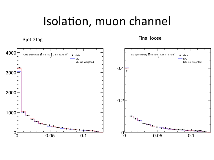
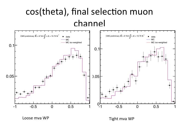
We have observed a small data-MC discrepancy in lepton isolation distribution. As it is difficult to estimate the QCD contribution for the isolation variable (the data driven estimate is derived in anti-isolated region), we have checked the lepton isolation shapes in 3j2t and 3j1t control regions, where the QCD contamination is minor. 3j2t sideband was used to extract event weights of (data yield)/(sum MC yield) in 3 bins of lepton isolation. Such weighs introduce no visible effect in the final cos-theta shape and we conclude that the related systematic effect is negligible.

     - line 306 : could you better justify the CompHEP/Powheg
comparisons for getting that systematic ? You could put there the
arguments you gave on the twiki.

The recipe of comparing with Comphep has been borrowed from the cross section measurements in this same channel. It has to be remarked that Powheg and Comphep have very different models for the signal: Powheg is a true NLO generator, while Comphep is LO but mimicks the main NLO effects by a matching procedure based on the pt of the associated "second b".

Did you consider a top-mass related
systematics ?

The top mass uncertainties have been incorporated and they actually have a not insignificant effect on the shapes in the signal enriched region, as is demonstrated in the following plot. However, for the cos-theta variable shape, they are not dominant.

     - line 321 : "top-quark mass"

OK

     - line 333 : "MC data" ? MC or data ?  I guess you meant something
like "limited amount of simulated events " ?

Yes. Corrected.

     - line 342 : "We also ...".  I'm not sure I understand the point
here. Could you try to be more precise ?

We wanted to test whether, by adding/removing a source of systematics, the central value moves significantly, and the test was successful (it doesn't move significantly, for any systematic).
But this is sentence is probably confusing, so we just removed it from the PAS (the information is in the AN anyway).

     - Figure 5 : nice plots !!! If I want to be picky, I would say that
the legend is too small, and that the "CMS prelim..." is not readable.

Thank you for the useful suggestions, which have been taken into account.

     - eq (8), could you use the format => value +/- (stat.) +/-(syst) ?

It will be done in all future drafts.
In the meantime, for the current results: A_l = 0.41+-0.03(stat)+-0.14(syst)

     - Figure 6 : do I understand correctly that the excluded areas are
within the colored regions ?

It's the other way around, the area allowed by the fit (at 68 or 95% CL) is within.

Point 1 on the twiki :

     - in the Mt(W)/MET fit, could you please show the distributions for
each processes separately and normalized to 1. This is to check the shapes.

• JA : Why do you merged to merge top (I guess ttbar+single top?) and QCD ? Looking at the plots, the QCD and DY seem to be much more similar. This is true for both channels and mT/MET
  • In the Mt(W)/MET fit, we do not merge top and QCD, this is done in the BDT fit. Instead, the components are 1) QCD 2)W+jets and 3) everything else

* Muons:

* Electrons:

     - Did you account for any uncertainty on the  merging of samples to
construct the templates ? Like an uncertainty on the fraction of ttbar
in the Top+QCD template for example ?

We have added a 100% uncertainty on the fraction of QCD in the Top+QCD template that we will propagate through the unfolding. Other samples (s-channel, tW-channel, DY+jets and Dibosons) get a conservative 50% uncertainty on their fraction. The effect is negligible for all but QCD.

     - The data/MC agreement for the electron channel is clearly
improved. However, there is still an excess of data for 3 bins
consecutively between -0.8 and -0.5? If this is just a statistical
issue, I suggest to use a different binning for that plot (Rebin(2) or
even (3)), this should also smoothen the MC distributions, which show
also some statistical fluctuations.

After evaluating the shape effect of all the systematics, the discrepancy seems to be contained, as can be seen on the plot below. It is fully contained when taking into account the normalization uncertainties, of which W+jets has the most significant contribution, followed by JES.

Comments on the AN, version from the 10th of August :

     - b-tagging SF : with you procedure, do I understand correctly that
you applied b-tagging SF considering the b-jet efficiency (inclusive/per
event) in MC signal events ? So you assume a certain pT/eta spectra ? Or
you are still considering pT/eta dependence of the SF ? If you use
inclusive SF (not depending on pT/eta) how can you be sure that it is
still valid for background processes ? Did you included an additional
systematic sources to account for these differences ?

We use pt and eta dependent scale factors as they are published by the b-tagging POG [1-2]. Consequently, we also measure and apply pt and eta dependent efficiencies for b-tagging and mis-tagging. The b-tagging systematics are calculated by propagating the uncertainties of the scale factors through the weight recipe which takes into account the combinatoric probability of tagging the jets.

[1] https://twiki.cern.ch/twiki/bin/viewauth/CMS/BtagPOG#2012_Data_and_MC_Moriond13_presc

[2] https://github.com/HEP-KBFI/stpol/blob/master/CMSSW_5_3_11/src/SingleTopPolarization/BTagSystematicsWeightProducer/src/BTagSystematicsWeightProducer.cc#L131

     - Could you check with the BTV group that you are using the last
up-to-date SF/efficiencies ?

We have now updated to the latest 22Jan ReReco SF-s [1]. We didn't do before, because BTV-13-001 had not been approved yet.

[1] https://twiki.cern.ch/twiki/bin/viewauth/CMS/BtagPOG#2012_Data_and_MC_EPS13_prescript

     - line 245 : I thought you apply the MET-phi corrections ?

We have checked the effect of the MET-phi corrections, and the effect of the correction on the BDT output and the cos θ is covered by the statistical errors. Anything shown thus far does not have the MET-phi corrections applied. Given that the effect on the analysis turns out to be negligible, we consider to stick to the Top PAG recommendations (which do not include the MET-phi corrections) for two reasons:
- uniformity with similar analyses in the same analysis group
- we are not totally sure about the correctness of these corrections for MC: while MET-phi becomes flat as expected in data, in MC there seems to be just a change in modulation, see this thread by Nadjieh and Orso who independently observed the same. See also slides 9, 11, 13, 15 of this talk, for a very different analysis, where these corrections are applied and the same is observed.

     - could you provide a complete cutflow table : number of selected
events after each (consecutive) selection steps, for signal and
backgrounds ?

This has been added to the AN (post v7), and also to this TWiki (apologies for the crude way of doing this).

     - line 262 : just to be sure that I understand; N is the number of
reconstructed and *selected* jets and M the number of reconstructed,
selected and b-tagged jets N?

You are correct. We always count the jets that pass our quality criteria.

     - line 290-293 : you take the jet with the highest discriminator,
just for curiosity, what changes if you take the highest pt jet instead ?

This can be checked, but since the selected jet and its 4-momentum propagates down through the analysis, it means a rerun of the n-tuples, which is somewhat more time consuming.
One can compare with the plots of the cross section analysis by Orso et al. (TOP-12-011 and the corresponding AN, where the key plots can be found), where jets are assigned randomly whenever there is an ambiguity. The shapes are very similar for cosθ, our variable of interest.

     - Figure 2 : is it with MET-phi correction ? At low mass, the
shapes of the electron and muon channels are different, is it due to MET
resolution effects ? Or background components ?

This is without applying the MET-phi corrections. See comment above about the lack of influence of these corrections on the analysis.

     - Could you please show the distribution of the number of
reconstructed vertex PU distribution after selection, and including the
PU reweighting ?

We checked the number of vertices distribution before and after reweighting, taking into account the systematic variations in the weight in 3 regions by studying the normalized distribution of the number of observed vertices.

* 2J1T data against t-channel

* 2J0T data against W+jets

* 3J1T data against ttbar

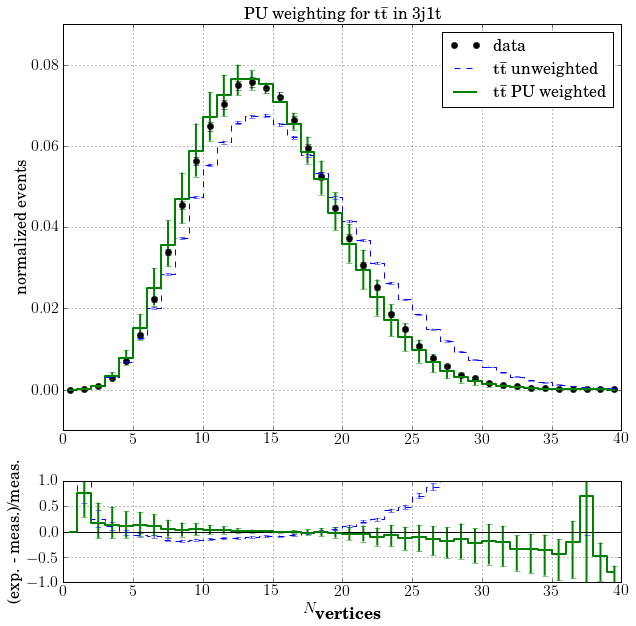The agreement is improved in all cases by the reweighting.

     - line 302 : as the ECAL integration windows is 300ns, is there no
out of time PU effect on the electrons ?

Indeed it is known, in the EGamma group, that the ECAL part of the isolation has a data-MC discrepancy due to OOT PU. This is supposedly corrected by the centrally-provided scale factors. We are now considering adding a shape uncertainty on the isolation variable (for both muons and electrons), see comments about the PAS above, and this should cover any effect from ECAL out-of-time mismodeling.

     - line 313 : Do you consider particles within the jets ? So within
deltaR=0.5 around the  jet axis ? Are you considering only charged
particles ? Or all PF particles ?

All PF particles.

     - MVA training : did you account for data-driven normalization of
backgrounds in the training ?

No, the training was performed without the normalizations as the normalization is derived later on the BDT discriminator output.

     - Line 342-343, how the mass of the jets are calculated ?

The mass is taken as the modulus of the 4-momentum of the jet, technically: ROOT::Math::LorentzVector::mass

     - Could you please show the over-training test : training performed
using halves of the signal and background samples, and tested on the
second halves. If there are no over-training, the output of the BDT for
signal and backgrounds should perfectly match.  Such a test is provided
by TMVA. This is a vary important check : I thought that the setting of
the MVA training might leads to over-training if you don't have very
large samples.

Electron channel:

Muon channel:

     - Figure 7 : there are some variables with high correlations. While
highly correlated variables are not necessarily a problem in themselves,
it is a bit dangerous if one doesn't check that the correlations are
also well described by the simulation. I would then try to remove these
variables and see how the Data/MC comparisons change for the BDT or to
check the correlations using data (but it might be non-trivial). For
example, pt(bj) and mass(bj) are highly correlated, and doesn't seem to
have large discriminating powers. So it should not hurt to much to
remove them.

As we already had various BDT trainings available based on the ranking of the variables and both of the variables in question (along with met and mass_lj) were at the tail of the ranking we could use a five variable BDT as a comparison. Find below the BDT discriminator output before the final fit. On the left hand side is the original full BDT and on the right the slimmed down BDT with less variables. Within the statistical fluctuations their data/mc agreement seems same.

• JA : Could you please specify which variables are used fr the alternative BDT training ?
• MK: The five variables are M(top), C, eta_lj, pt_lepton, MtW

Electron channel:

Muon channel:

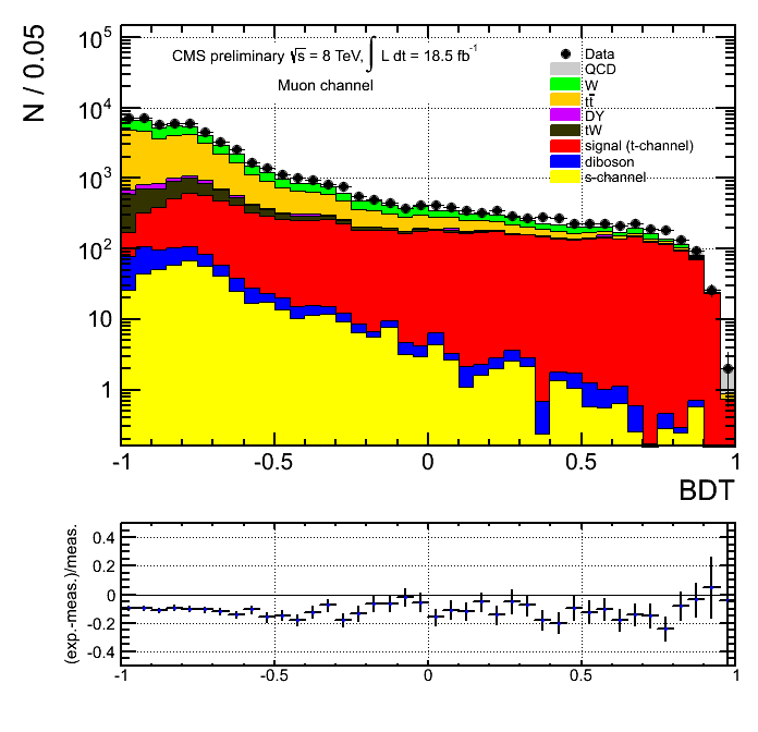
     -  do you used statistically independent samples for the training
and for the "reading" ?

The training of the BDT was done using the inclusive MC samples for W+jets and ttbar. However the reading and testing have been done using the exclusive samples. Therefore the samples are completely independent.

• JA : What about the signal ? Well, I don't think it is a big issue anyway.
• The signal is the same. We use inclusive samples for training and exclusive for testing.

     - Figure 8 : it is difficult to check the data/MC agreement in the
signal region (especially the (exp-meas)/meas. ratio) given the large
statistical fluctuation. Could you change the binning ?

Binning updated.

     - line 374 : 30% ?

Yes, simple typo in LaTeX where % is discarded as a command symbol. In fact it also removed a big part of a paragraph explaining the ranking procedure hence the understandable questions about the next paragraph.

     - Line 375 : "no such variables were found". I have no idea what
you are referring to. Could you be more explicit ? Line 377 : "that gave
the biggest worsening", how do you evaluate the "worsening "exactly ?

This means that removal of any variable from BDT produced a new BDT that had less background rejection at the same signal efficiency than the BDT with this variable still included. The worsening is evaluated by taking the ROC curve value at signal efficiency of 30% i.e. background rejection percentage. Therefore there is worsening of the BDT if at 30% signal efficiency the background rejection gets worse. The biggest worsening is for a variable for which the background rejection percentage drops most.

     - From line 371 to 382, I'm not sure I understood the idea behind
that check. Is it to check if the addition of one variable is worsening
the discriminating power of the BDT ? The BDT is known to be robust
against the addition of variables which has no strong discriminating
power. Or are you trying to check if the distributions are well agreeing
between data and MC (then I would not understand the section at all) ?

It is a consistency check to validate that all variables are adding to the power of BDT, this was requested previously as a sanity check even though indeed BDT is very robust about amount of variables.

     - Figure 10 to 27 : in the captions "right column is after the
final fit", does it means "after accounting for the normalization of
backgrounds determined from the template fit" ?

You are correct.

     - Figure 10 to 27 : I can not always look properly at the data/MC
ratio plots, because the range in y-axis is too small. Some Figures,
like the 14-15 ones, really need to be re-binned.

Re-binned and y-axis range extended to be +- 100% (i.e. -1..+1).

     - Figure 10 to 27 : what are the loose and the tight BDT cut ?
Which one of the two is used for the measurement ?

The loose cut is defined as the cut on BDT that for the signal sample gives about the same yield as the cut based approach. Originally BDT was developed as a second path and the working point allowed for best comparison while retaining about the same signal yield and therefore was ideal for check of how much this improves the result, especially the systematic errors. The tight working point was selected by eye to give a close to background free state, especially with regard to W+jets background (the source of largest uncertainties). However due to low remaining signal yield it isn't actually used besides a cross check to validate if some excesses might be background related.

In addition the actual plan is to optimize the BDT cut based on minimizing the total uncertainty. This process is currently in the works and hopefully can be shown in the very near future as this was the original plan with BDT to balance between the statistical uncertainty of ever reducing the signal yield vs the systematic uncertainties related to background processes. This however requires an iterative process of unfolding at every BDT cut value and evaluating the total uncertainty and therefore required more time, but should be available very soon.

     - Figure 11 : the mT (top mass) ? distribution seems to be narrower
in data compared to MC for the loose BDT cut, is it covered by
systematics on the shapes ?

This seems to be covered by the generous statistical uncertainties, of which the most important is the uncertainty in the top mass, followed by the uncertainty in the t-channel scale.

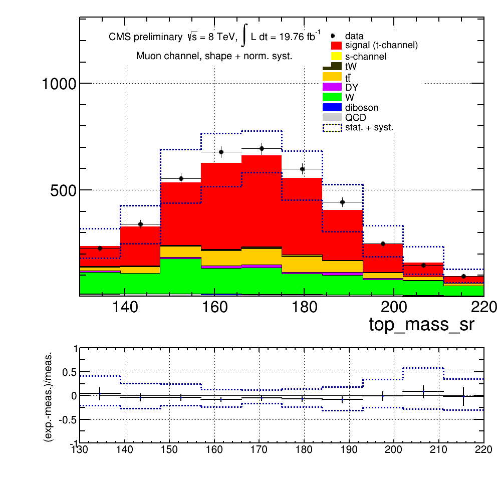
     - Figure 17 : there is clearly a trend in the MET shape for the 2
firsts rows. Do you have an explanation ? Is it because of QCD
contamination ? Why QCD has some events below 50 GeV ?
     - Figure 18 : there are clearly in some data/MC disagreement for,
especially at low Mt(W) values. This is a sign of QCD (fake-lepton)
contributions ? Again, why there is QCD events with Mt(W) > 50 ?

The way our plotting tool was created and configured caused an artifact for MET in electron channel and Mt(W) for muon channel. Namely the shape template was taken before the MET/Mt(W) cut and the yield was taken after the cut. This improved significantly the statistical shape of the QCD template and did provide better agreement across the board for most variables. However for the actual variable used for QCD rejection this breaks down because the template before cut will be different significantly for obvious reasons. However as those plots were generated through automatic tools this issue slipped in. The QCD estimation method through this template + yield method works fine for all other variables assuming they don't have a strong correlation to the MET/Mt(W) variable.

• JA : do I understand correctly tht the QCD events used later in the analysis are "data" events from a contrl region, without the MT and MET cuts for the muon and the electron channels respectively ? If yes, how the non-application of the cuts are affecting other shapes ?
  • We are now applying the MT / MET cut for taking the templates.

     - Figure 20-22 : there is an excess of events in the low pT region.
Again, is it related to some QCD contamination not shown properly ?

FIXME@joosep => WIP

     - Figure 26 : in the data/MC ratios, the dots are completely out of
range. I don't think this is just a normalization issue, especially for
the bottom plots, where clearly the shapes are different between data
and MC.

For readability the ratio plot was limited to +- 20%. However on some plots this is prohibitive and needs extending.

     - Figure 28 : those plots differs from the ones on the
PasTop13001QA TWiki page ?

These were based on an older iteration of the ntuples and have now been synced with the PAS.

     -Starting from line 440 : I don't understand why you are accounting
for uncertainties likes JER et JES (and MC statistic...) while you are
extracting the QCD multijet samples from data ? Is it applied on the
subtraction of other backgrounds in the QCD enriched region ? By the
way, did you accounted for a systematic on the normalization of the
subtracted backgrounds ? (you should).

Yes, they are applied on the subtraction of other backgrounds in the QCD enriched region and also for extracting templates for other processes besides QCD (the rest are taken from MC). After the fitting, we assign a conservatice uncertainty of 100% to the QCD yield, so also the normalization of the subtracted backgrounds will be accounted for by this.

     - the fitting procedure in the AN seems to use 4 templates, while
on the twiki you use 3. I guess the AN was not updated ?

Indeed, we changed the procedure following your comment at the preapproval, and the AN was not updated yet when you wrote this new set of comments.

     - table 7 : in that table, are the data-driven normalization of
backgrounds from the BDT fit included ? I guess not given the large
differences there is between data and predictions. I would include those
scaling factors in order to show really the data/MC agreements you have
right before performing your measurement. I would also account for the
corresponding uncertainties.

See reply in the next round of questions.

     - Line 506-507 : Is the reweighting applied after the event
selection or before any event selection ? Because what you do seems to
be equivalent than just using sherpa but after normalizing it to the
MadGraph prediction;

Weights are extracted before any selection, and applied to selected events. Here we only consider the shape effect.

     - Line 510-511 : if the reweighting is applied before the event
selection, you should check that all the variables used in the event
selection, and the BDT training, are not affected. Not only the eta_j
variable.

We did the check in the signal region and all differences were well within statistical uncertainty.

     - Section 5.3.2 : Just to make sure I understand : you just take
the QCD normalization from the Mt(W) and MET fits, and fix it for the
BDT fit ? But with the Mt(W) and MET fits you also somehow estimated the
normalization of other processes. Are they found to be compatible with
the output of the BDT fit ?

In the BDT fit we use the value from the QCD fit as the central value with a 100% uncertainty.

Below is the comparison of the results from the 2 fits. It has to be noted that the templates in the 2 fits contain different components so the results are not directly comparable. However, you can see that in the electron channel the resutls are compatible. There is a discrepancy in the muon channel, but it can be attributed to the similarity of W+Jets shape with other MC shapes in the QCD fit. To cross-check the BDT fit, we have performed the fit also on the variable "C" and the results agree with the BDT fit.

Electrons:

• QCD fit
  • W+jets: 1.90 +- 0.18
  • Other MC: 0.96 +- 0.05
• BDT fit
  • t-channel: 0.86 +- 0.06
  • top+QCD: 0.82 +- 0.11
  • W/Z+jets, 2.18 +- 0.32

Muons:

• QCD fit
  • W+jets: 1.26 +- 0.13
  • Other MC: 1.14 +- 0.05
• BDT fit
  • t-channel: 0.99 +- 0.04
  • Top+QCD: 0.82 +- 0.09
  • W/Z+jets: 1.92 +- 0.21

• JA : I'm a bit confused. What should I compare ? In the QCD fit, the "QCD" is within "other MC" ? In the numbers quoted above, is the uncertainty statistical only ? I'm not expecting the QCD SF to be the same in the electron and muon channels, but other SF should be compatible. This seems to be the case ?
  • No, in the QCD fit, the QCD is a separate category. The fitted value from QCD fit is used as input for BDT fit, so as we assign a 100% uncertainty to it, the scale factor would be 1.0 +- 1.0. Sorry about not being clear about that. The uncertainty is statistical only

     - Line 564 : are there some systematics on the fractios of each
process which constitute the template ? Same question for template on
line 566.

We have added a 100% uncertainty on the fraction of QCD in the Top+QCD template that we will propagate through the unfolding. Other processes (s-channel, tW-channel, DY+jets and Dibosons) get a 50% uncertainty on their fraction. The effect is small for everything except QCD.

     - Line 702 : what is the justification of the 10% uncertainty on
ttbar ?

The 10% uncertainty was on merged ttbar, s-channel and tW-channel. Now that we added QCD to this group the uncertainty is set at 20% as the prior uncertainty on QCD is 100% and there is roughly 10 times as much top events as QCD. We can see that ttbar is quite well modeled so 10% seems reasonable. To check, we set the top+QCD component prior uncertainty to 100% and fit again. The resulting rates are stable in both channels, the largest change being in W/Z+jets rate, but still under 1%. The signal scale factor changes less than 0.1%

• JA : I personally found 10% a bit too small. This is barely the theoretical uncertainty on the cross-sections ? From the check you performed, do I understand correctly that the result of the fits is not changing bu more than 1% for every components ? How far the top+QCD nuisance parameters moved from its initial value ? To me, it is rather that 100% QCD is over-conservative, so it might well compensate the any possible under-estimation of the top-related uncertainty. But all in all, your check seems to be conclusive, so it should be fine.
  • Yes, you understand correctly that no component changes more than 1%.
  • The uncertainty on the measured cross section value is well below 10%.
  • For the systematics, the difference between 20% and 100% uncertainties can be bigger than for nominal, often around 10% difference.

     - Line 711-713 : I don't understand the point. There are no
uncertainties on the "other backgrounds" ? Even if they are part of the
templates, they should have an effect, that needs to be quantify. For
example, if you vary the fraction of diboson events by 50%, does it
affect the BDT fit and thus the final result ?

We have added a 100% uncertainty on the fraction of QCD in the Top+QCD template that we will propagate through the unfolding. Other samples (s-channel, tW-channel, DY+jets and Dibosons) get a 50% uncertainty on their fraction. The effect is small for everything except QCD.

JA : I'm confused again. Earlier you were speaking of 10% for s-channel, tW-channel and ttbar ?

• The 10% (or 20% for Top+QCD) is the uncertainty for the whole template.

50% is the variation of the small components in the merged template (s-channel fraction in the Top+QCD template, etc.), like you asked

     - Figure 52 : the bottom plots are not only re-normalized to 1 ?
Because the shapes are different. Is there a typo in the legend ?

FIXME

     - Table 10 : when will it be completed ?

Done.

     - Figure 55: I don't understand which pseudo-experiment are in
there. Could you explain to me how these plots are made ?

Now added to the PAS text.

     - section 9 : I'm not sure what the TopFit program do exactly. To
my understanding, it is performing a multi-dimensional scans of the
parameters of the effective lagrangien (23), calculating the various
observables for each benchmark, and calculate the limits out of the
scan. It is not clear to me how the limit is exactly computed  from the
numbers in table 12 and the scans. I also want to make sure you didn't
used it as a black-box.

TopFit works as follows: Anomalous couplings and the polarization are diced uniform in the range indicated in table 11. From each diced set of couplings and polarization, the theoretical expected values (obsTheo) for the observables can be calculated. In detail this is

- the W helicity fractions (F+, F-, F0) which can be expressed in terms of anomalous couplings

- the spin-analyzing power (alpha_l) which can also be expressed in terms of anomalous couplings. The asymmetry is obtained by multiplying the spin-analyzing power with the independently diced polarization

- the single top cross sections. Their dependence on the anomalous coupling was determined and parameterized by the TopFit author with the event generator PROTOS.

TopFit calculates then over all observables the sum of (obsTheo-obsMeasured)**2/sigmaMeasured**2. For the W helicity fractions, the measured anti-correlation is taken into account as well. The diced point in the coupling and polarization space is then accepted according to its probability of the resulting chi2 distribution. The procedure of dicing, calculating the observables and the chi2 is currently repeated 3,000,000 times to obtain a dense point cloud for the limit plots.

     - also, it is not obvious to me that the measurements presented in
table 12 should be treated as independent.

Unfortunately TopFit doesn't allow to take correlations into account, and although we already informed its author that we would like this feature, it is unlikely to be available soon.
However, we can argue that correlations are not large, upon the following arguments:
- the single-top cross section and the W-helicity come from the 7 TeV dataset, while our measurement is at 8 TeV
- the W-helicity number comes from the CMS+ATLAS combination, therefore ATLAS data dilute the correlation with the other two which are CMS-only
- the W-helicity number comes from ttbar combinations (the W helicities from the single-top selection is not included in this average), hence a selection which is orthogonal to the other two.

We are aware that some kinds of systematics are anyway correlated across these measurements, but at first order the approximation of independence should be a good one.
Moreover, the same assumption of independence between single-top cross section and W helicity has been used by all the W-helicity measurements, when showing the limits on anomalous couplings taking into account the constraint from single-top cross section.

• JA : I tend t agree, only if all the measurements are dominated by statistical uncertaintes, and/or by systematics which are not related to JES/JER/Btag/signal modeling (etc...). Is there a way to check this quickly ? Anyway, I would explicitly mention in the PAS that this is a feature of TopFit.
• AG: for the moment I just added more text to explain that correlations are neglected, that this is a feature of TopFit, and some heuristic explanation to say why they are probably not an issue. Contacted Mara to see if she has some good suggestion about how to quantify the effect of correlated systematics across these very different measurements.

The following points should be addressed before handing the analysis over to the ARC:

1) Understand better the unexpected result of the QCD fit in electron channel

Some checks or modifications that we did:

a) Added a systematic uncertainty on QCD shape by varying the anti-iso cut used to extract the template; no effect on the result.

b) Added a systematic uncertainty from the limit statistics of the templates (which was not correctly propagated to the final result before); therefore the total error bars enlarged a bit (from 0.07 to 0.08).

c) As suggested by Jeremy, we decreased the number of fit parameters; we chose to merge Top and QCD, as we had discussed at the meeting, upon the argument that they have very similar cosTheta shapes (and also similar BDT shapes by the way), and this had quite an effect on the scale factors, which now agree very well across the two channels:

Category	Muon channel	Electron channel
Signal	1.03+-0.06	0.96 +- 0.08
Top+QCD	0.91+-0.11	0.98 +- 0.14
W+Z+VV	1.60+-0.24	1.38 +- 0.43

This has to be compared with slides 22 and 23 of the preapproval talk, where the signal from the fit was very different between the two channels.

It can be concluded that now the two channels give results in agreement for all the categories. Moreover, in the muon channel the new result is not very far from the old result.

Now the cosTheta data/MC comparisons looks like that, after normalizing to the new fit results (with a systematics band that takes into account, on purpose, only the shape effects):

For comparison, these are the same plots with the old scale factors (as in the preapproval talk):

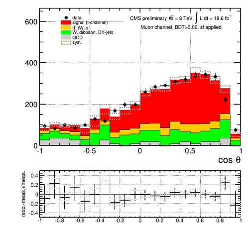
Conclusion: the shape difference between data and MC for electrons is now mostly covered by the shape systematics, while this was not the case before.

2) Vary initial cuts on MT / MET cuts and check effect on cos(theta*) shape

We performed the following checks:

a) applying a MT cut of 30 GeV, instead of 50 (muons, left) and a MET cut of 30 instead of 45 (electrons, right):

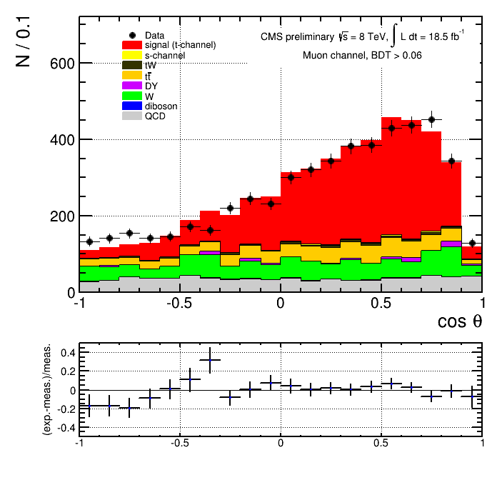
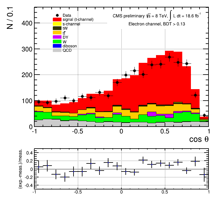b) applying a MT cut of 50 GeV (the top reference selection) and a MET cut of 50 instead of 45 GeV (for the sake of coherent cut values for this particular comparison):

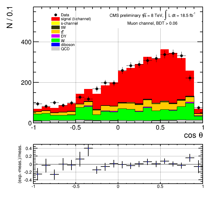
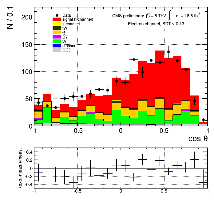c) applying a MT cut of 70 GeV, instead of 50 (muons, left) and a MET cut of 70 instead of 45 (electrons, right):

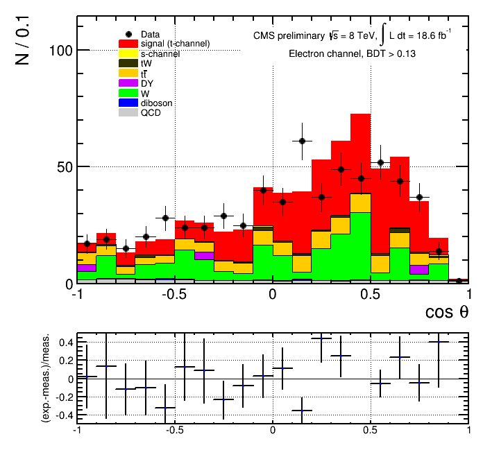Note: the scale factors have now been derived for each particular region, by considering the 3 categories: t-channel, top+QCD and W+diboson separately and 3 MET/MT cuts separately. LIkewise for the QCD estimation via the MET/MT fit.

Category 30 GeV	Muon channel	Electron channel
t-channel	1.06 ± 0.06	1.16 ± 0.10
top+QCD	1.02 ± 0.10	1.05 ± 0.17
W, diboson	1.30 ± 0.21	1.21 ± 0.31
Category 50 GeV	Muon channel	Electron channel
t-channel	1.03 ± 0.06	0.87 ± 0.07
top+QCD	0.91 ± 0.11	0.95 ± 0.12
W, diboson	1.60 ± 0.24	1.47 ± 0.39
Category 70 GeV	Muon channel	Electron channel
t-channel	0.88 ± 0.09	0.75 ± 0.11
top+QCD	0.76 ± 0.13	0.74 ± 0.15
W, diboson	1.96 ± 0.31	2.32 ± 0.64

Conclusion of a,b,c: the data/MC agreement does not depend on the tightness of the anti-QCD preselection cuts.

We have internally discussed about the variation in scale factors between different MT/MET cuts. It's important to know that the BDT was not re-trained for each case, therefore it is sub-optimal whenever preselection cuts are changed: wit a looser preselection, the BDT has to take a decision about new data from a kinematic region that it has never encountered during training, while a tighter selection makes all the three categories more similar to each other than they were in the training set (and moreover, the internal background composition is different than during the training). In both cases, we get less discrimination for the BDT, and therefore larger degeneracies and larger uncertainties.

d) replacing the MET cut with a dedicated BDT (which includes MT and MET among its inputs) for signal/QCD discrimination:

This BDT has been trained with 2j0t events, to get sufficient statistics, and QCD events for the training have not been taken from MC but from anti-iso data. A cut of BDT larger than 0.74 is applied, chosen such to give the same signal efficiency as the MET cut. The above plot is without final fit coefficients. The QCD template is extracted from data, as usual. As a cross check, below is the same MVA distribution in the anti-isolated region:

(In this plot there is no histogram for the "QCD expectation", as MC has no sufficient statistics for this tight selection, even in the anti-iso region, and therefore we take our QCD expectation from this anti-iso region in data.)

The cosTheta plot after this cut is:

And the final cosTheta plot after applying also the MVA cut trained against W and top backgrounds is:

Conclusion: a specialized anti-QCD MVA gives a rather good agreement in the signal region. This could also be a replacement for the MET cut in the future.

3) Provide (preliminary) table of systematic uncertainties

Done, in the next version.

4) Update PAS with latest results

Done, in the next version.

Equation (1) : what is meant by forward/backward here ? Are you
referring to spin axis ? Up and down arrows could be more explicit ?

Your understanding is correct. We like your suggestion of using arrows.

Section 3 : was trigger and lepton efficiencies measured in data and the
corresponding SF applied to the simulation ? I see a systematic on this
(line 315) but it is not explained in the text ?

Yes they are. The AN provides the sources of the numbers. We are adding a sentence in the PAS, thanks for pointing that out.

Equation (5) : Is the \Lambda single top cross section ? I guess it
compares to equation 5.2 of arXiv:0805.1333 ? If this is the case, is
there not a factor 1/2 missing in the right term of equation (1) ?

Do you mean \Gamma? If so, it is the partial decay width. In the same review paper that you are citing, you can find exactly the same formula in eq.3.11; we could have written as in eq. 5.2 of that paper, but even in that case, the right-hand side would be correct because we are choosing a notation where A_l is half of P_t*α, differently from that paper.

Figure 1 : clearly, there seems to be a trend in the cos theta*
distribution. There is an excess of data in the low BDT region and a
deficit in the high BDT region. It it covered by a shape
uncertainty(ies) ?

If you talk about the BDT distribution, actually its ratio is rather consistent with flatness.

Instead, it is true that the cosTheta shape is more flat than predicted by our model. Among the possible reasons there are new physics (which would give exactly that kind of flattening) and an underestimation of backgrounds. But the posterior uncertainty from the fit covers the discrepancy, see figure below:

In principle no detector uncertainty affects cosTheta significantly (we are producing some plots to demonstrate that, it will be for the next drafts), with one possible exception: MET-phi modulation, that we don't consider yet. We realized that the MET-phi corrections were not applied, and we are now reprocessing all data and MC (not in time for preapproval). There are qualitative indications that the effect goes in the direction of improving the data/MC agreement of cosTheta itself, but we will be able to quantify only at the next iteration.

If I understood well, there are no scaling factors nor the associated
uncertainties accounted in the numbers presented in table 1. There is a
very large difference between data and MC, especially for the muon
channel. Is it understood ? Looking at the table 2, is seems that most
of the difference could be explained by the SF of the signal? But why
this is not the case for electron channel ? In that case, the SF for
signal is closer to 1. Shouldn't it be the same ? Or is there some kind
of electron-related selection which is including some differences ?

Standard scaling factors (but not their uncertainties), like lepton selection, b-tagging, etc., are applied in table 1. Part of the discrepancy may come from the RMS cut (you can see plots in the AN) which is discrepant, and may indeed be removed in a next iteration of this analysis.

Muon and electron channel apply different selections, most notably:

1) MT cut for muons, MET cut for electrons

2) different lepton threshold

So in principle the scale factors can be different given the different phase space. Moreover, we have indications that the MET-phi corrections (to be applied at the next iteration) will have different effects on the two channels, and we understand this by point 1), i.e. the fact that the MT and MET variables have different correlations with MET-phi.

I would also rather show table 2 after applying the SF for backgrounds.

Do you mean scale factors on the standard MC-to-data corrections? These are applied.

Section 5.2 : MadGrap vs Sherpa. Just to make sure I understand : the
Madgraph W+jets sample show some discrepancies in the 0Btag region, but
sherpa does described well the data ?

You understanding is correct. Sherpa describes the shape better in 2j0t.

But you don't want to use Sherpa because it affect the number of bjets.
Instead you use the costheta* distribution from sherpa to reweight the
costheta* distribution in MadGraph. Did I understood correctly ?

Your understanding is correct.

As you are using a BDT, did you make sure that other distributions,
especially the ones used in the BDT training, are not getting worse
after the reweighting ?

In the next version of the AN you will see the data/MC plots for all the individual inputs after this correction, showing very nice agreement. We prefer not to show include the plots also before this correction, to avoid cluttering the note even more. However, in the signal region the difference turns out to be negligible.

Figures : there are many (maybe too many ?) control plots, but no plots
in the signal region except for the BDT ones. Was every observables used
as input to the BDT checked in the signal region as well ?

See answer above: it will be in the next AN draft.

By the way, we are also reducing the number of plots in the PAS for the control regions.

For the ttbar background, did you applied the top pT reweighting from :

https://twiki.cern.ch/twiki/bin/viewauth/CMS/TopPtReweighting

and propagated the corresponding uncertainty ?

We will include it as an additional systematic in the next draft. We expect a negligible effect, though (it only affects ttbar, not the signal, and we expect the shape of cosTheta to be very resilient against any pt variation of the analysis objects.)

Line 322 : I'm pretty sure there are btagging SF available for 8 TeV.
You should definitely use those.

Are they already recommended for use in analysis, even if BTV-13-001 is not approved yet? (The current flag on CADI is "preapproved".) We will make sure that the new SFs will be available at the next iteration, in order to quickly switch to them as soon as BTV-13-001 is approved.

Line 340 : the "signal generator" uncertainty is quite unclear to me.
Which kind of uncertainty exactly are you trying to estimate ? I don't
think that comparing 2 generators give necessarily a good (nor a
conservative) estimation of the signal modeling uncertainties. I would
rather use a single generator and vary its parameters. I think there
something like a "scale" parameter in pohweg for example. And
powheg+pythia and powher+herwig could be used for estimating the effect
of showering. But I guess such studies would requires some MC production
as most likely these samples are not existing?

We are already considering a variation on Q^2 in Powheg. Unfortunately, as you point out, other kinds of comparisons (like pythia vs herwig showering) are unfeasible on this timescale for lack of samples. The recipe of comparing with Comphep has been borrowed from the cross section measurements in this same channel. It has to be remarked that Powheg and Comphep have very different models for the signal: Powheg is a true NLO generator, while Comphep is LO but mimicks the main NLO effects by a matching procedure based on the pt of the associated "second b".

For the BLUE combination. I'm not sure it is correct to treat the
backgrounds as uncorrelated between the electron and muon channels. This
is because the same simulations are used in both case, even if the SF
are determined separately. Thus, the correlation is probably not 100%,
but certainly not 0% neither. I suggest you try these two extreme cases
and take the one which leads to the highest uncertainty, to be
conservative.

We will consider how to take this into account in practice. What we call "stat+bkg" uncertainty is the statistical uncertainty from the unfolding, where the unfolding is performed after the "uncorrelated background subtraction" procedure, therefore the two kinds of uncertainties are totally entangled. A possible way to disentangled them could be to use toy data diced from a toy MC model where no background is included. Once we know the effect of the backgrounds on the "stat+bkg" uncertainty, we can play with its correlation in the combination. What do you think?

Figure 5: I guess the plots are not finalized yet ? The left plot is
very confusing and the unfolded and generated distributions are not
agreeing very well.

Indeed. We are sorry for the placeholders of the current version, we plan to have final plots at the preapproval.

I need to go through the anomalous couplings part in details (sounds
good !) but it would be great to remind the current limits on anomalous
Wtb couplings, so the reader could compare the current limits to the
already existing ones.

We chose not to do that, because the next-to-last figure is already showing the difference between pre-asymmetry and post-asymmetry fits in several 2D slices of the 5D space of parameters. But if you think that it would be more informative to add some numbers in the text, we will do.