Object selection
More  Less
Less  More Less
Leptons
Leptons are reconstructed in the following way:
- electrons -
pixelMatchGsfElectrons
- muons -
globalMuons
Observables for leptons
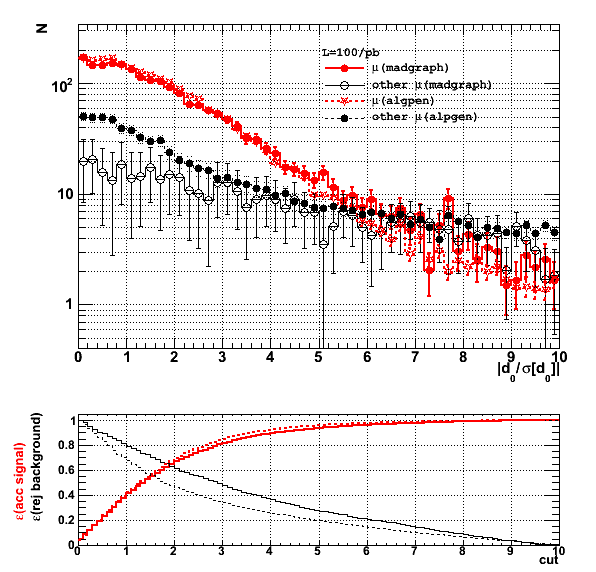
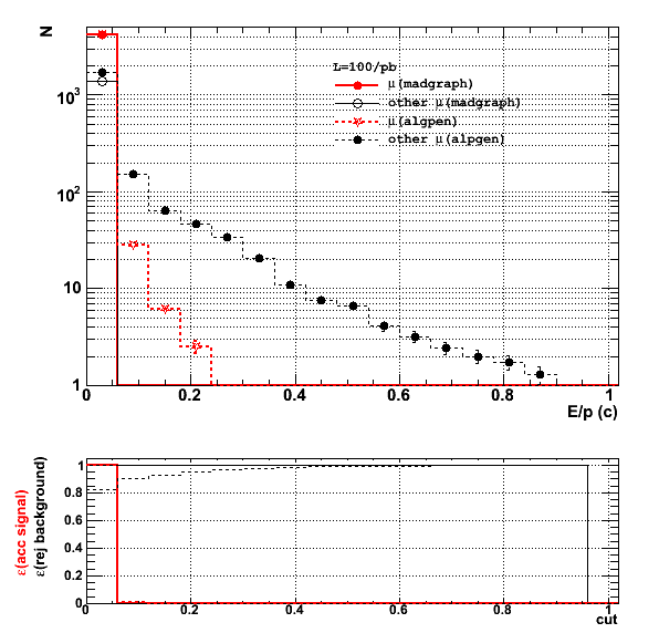
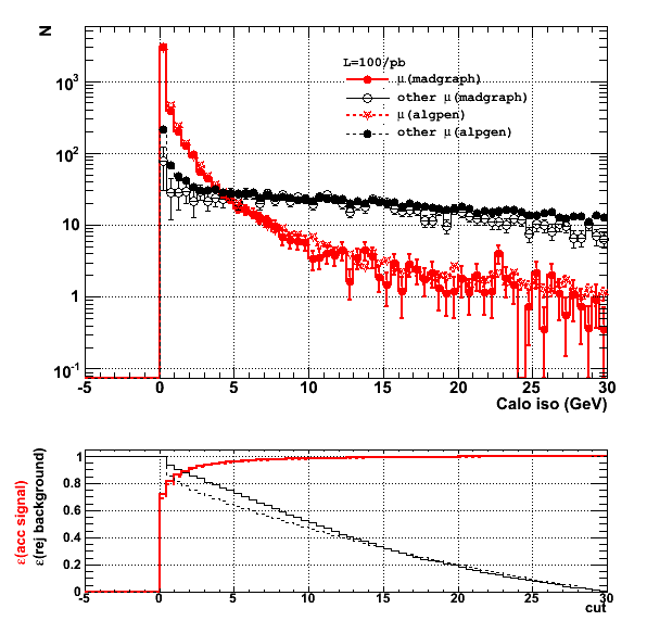
The main characteristic for leptons coming from the W decay is the fact that they should be prompt and isolated. Other variables can be used to clean the leptons of interest: electromagnetic fraction, E/p, lepton identification, etc.
| Reconstructed lepton observables |
| |
 spectrum spectrum |
 distribution distribution |
Track impact parameter |
 |
| e |
 |
 |
 |
 |
 |
 |
 |
 |
 |
| |
electromagnetic fraction |
Isolation in tracker and calorimeter |
|
| e |
 |
 |
 |
|
| |
 |
 |
 |
|
Single lepton selection efficiency and purity
Our lepton selection is defined below.
| Lepton selection |
| Selection steps |
Electrons selected |
Muons selected |
| kinematics |
 ; ;  |
 |
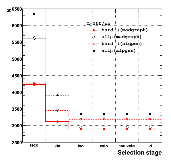 |
| calorimetric cuts |
 |
| isolation |
 |
| id |
 |
After selection the lepton purity is the following:
| Sample |
Leptonic purity |
| e |
|
Madgraph |
1.00  0.02 0.02 |
0.98 0.02 |
Alpgen |
0.96 0.01 |
0.952 0.005 |
| Purity |
0.96 0.01 (stat) 0.03 (syst) |
0.952 0.005 (stat) 0.03 (syst) |
The probability of reconstructing and selecting both hard leptons is the following:
| Sample |
P(select n hard leptons) |
| 0 |
1 |
2 |
Madgraph |
0.240 0.004 |
0.487 0.006 |
0.273 0.004 |
Alpgen |
0.227 0.001 |
0.483 0.002 |
0.290 0.002 |
 |
0.227 0.001 (stat) 0.013 (syst) |
0.483 0.002 (stat) 0.004 (syst) |
0.290 0.002 (stat) 0.018 (syst) |
Jets
Jets are reconstructed using the iterative cone algorithm with  from the calorimetric towers with
 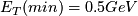 . A minimum
  of 2 GeV and 2 towers is required as pre-selection. The tracks with at least 8 hits, a
  and
and  are associated to the calorimetric cluster if they are matched to it within a cone of . No jet cleaning (matching with reconstructed electrons or muons is done).
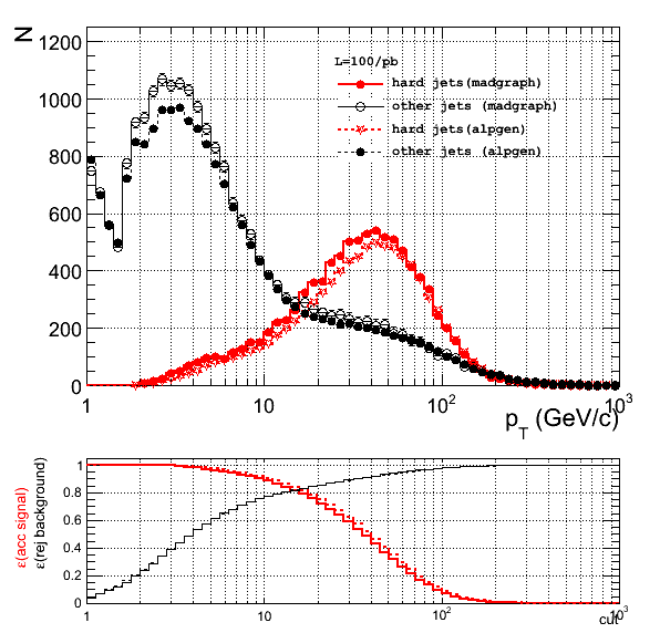
Observables for jets
| Reconstructed jet observables |
| spectrum |
distribution |
emf |
b-tag discriminator |
 |
 |
 |
 |
| Calorimetric constituents |
Associated tracks |
 |
 |
 |
 |
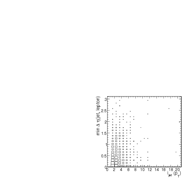
| nearest jet |
|
|
|
|
 |
|
|
|
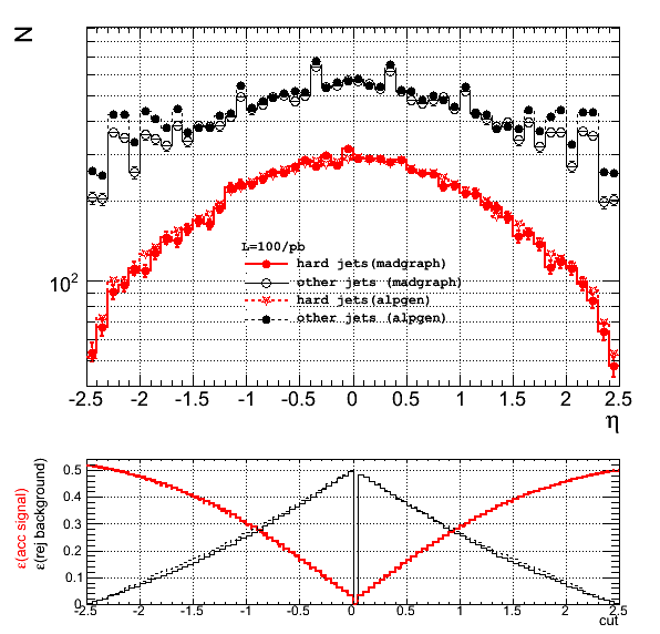
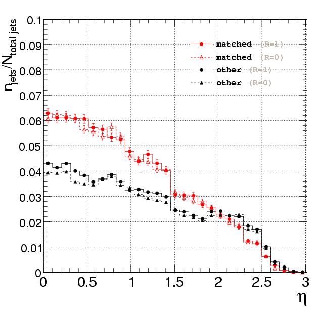
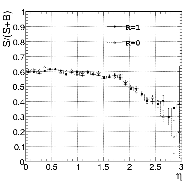
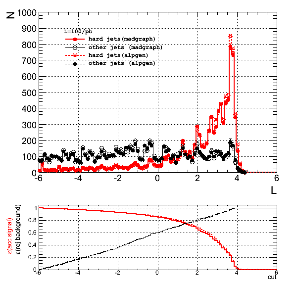
Likelihood ratio method
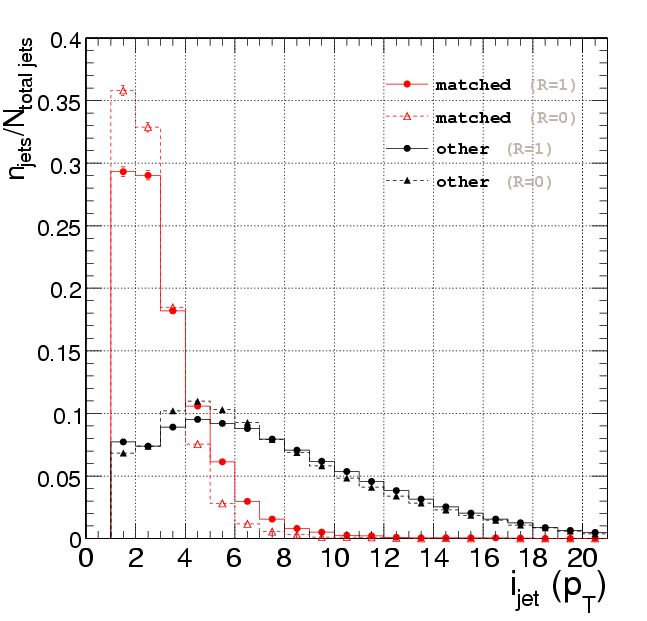
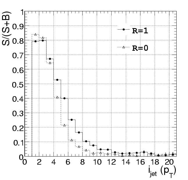
In order to increase the purity of the jets selected in an event we try to characterize better some experimentally measurable distributions of the jets (e.g. jet width, number of tracks, charge, etc.). For each jet we compute a list of observables and we check if it can be matched to the quark generated by the top decay (b,s or d ). This allows us to define two distributions:
-
 - the "signal" distribution for the jets whose purity we want to increase.
-
 - the "background" distribution for the jets remaining, after the selection, which you want to remove.
The distributions S(x) and B(x) are defined with inclusive first and last bins. As so, the first(last) bin should be interpreted as the number of jets with an observable x ,  (
( ). The probability distribution function -
 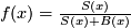 gives the probability that a signal jet has an observable x between x and x+dx.
Having defined the p.d.f.'s for signal jets one can define the combined likelihood as:
In order to reduce possible bias sources the different p.d.f.'s must:
gives the probability that a signal jet has an observable x between x and x+dx.
Having defined the p.d.f.'s for signal jets one can define the combined likelihood as:
In order to reduce possible bias sources the different p.d.f.'s must:
- have low correlations (
 )
)
- not bias towards the selection of a specific jet flavor (b,s,d)
The table below summarizes the distributions for the observables chosen and the correspondent likelihood obtained when using Madgraph (All b and All q samples).
| Jet properties |
| x |
S(x) and B(x) |
 |
Cross correlations |
 |
 |
 |
 |
 |
 |
 |
 |
 , number of towers with , number of towers with  of the jet energy of the jet energy |
 |
 |
 |
 , jet index in a ordered jet collection , jet index in a ordered jet collection |
 |
 |
 |
 |
 |
 |
 |
| Combined Likelihood |
| likelihood |
signal efficiency vs. background efficiency |
 |
 |
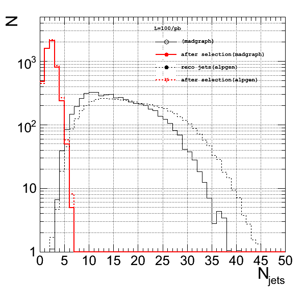
Single jet selection efficiency and purity
Our jet selection is defined below
| Jet selection |
| Selection steps |
Jets surviving selection |
Multiplicity |
Likelihood (after pre-selection) |
| kinematics |
;  |
 |
 |
 |
| calorimetric cuts |
 |
| topology |
 |
| likelihood |
 |
After selection the jet purity is lower than lepton purity (as expected due to the high jet multiplicity):
| Sample |
Jet purity |
Madgraph |
0.726 0.007 |
Alpgen |
0.725 0.003 |
| Purity |
0.725 0.003 (stat) 0.01 (syst) |
The probability of reconstructing and selecting both hard jets from the top decay is, however higher than the one obtainde for leptons:
| Sample |
P(select n hard jets) |
| 0 |
1 |
2 |
Madgraph |
0.137 0.003 |
0.427 0.005 |
0.435 0.005 |
Alpgen |
0.124 0.001 |
0.425 0.002 |
0.451 0.002 |
| |
0.124 0.001 (stat) 0.013 (syst) |
0.425 0.002 (stat) 0.003 (syst) |
0.451 0.002 (stat) 0.016 (syst) |
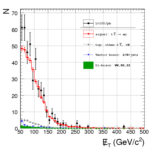
MET
In the di-leptonic channel the missing transverse energy has two main sources:
- neutrinos emitted by the decay of the W's generated by the top decay
- neutrinos emitted in the leptonic decay of
 's
's
The spectrum of the MET reconstructed by the corMetType1Icone5 algorithm, after selecting at least 2 leptons and 2 jets, is shown below:
 Our MET pre-selection is defined as: MET > 50 GeV .
Event selection
Trigger
We require a or of HLT trigger bits dedicated to single leptons:
-
HLT1ElectronRelaxed
-
HLT1Electron
-
HLT1MuonIso
-
HLT1MuonNonIso
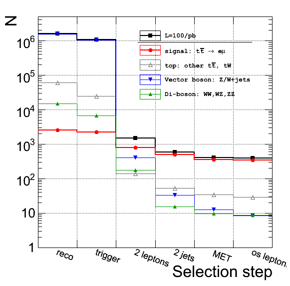
Selection
The table below summarizes the event selection used for the di-leptonic channel:
| Selection step |
Constraints |
Event selection |
 |
or of HLT trigger bits for single leptons |
|
 2 leptons 2 leptons |
;  |
 |
| |
| |
| id : |
| 2 jets |
; |
| |
| |
| |
 |
 |
| op. sign leptons |
 |
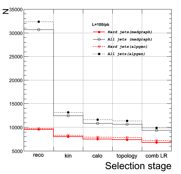
The table below summarizes the events surviving each selection step (computed from the CSA07 samples).
| Total events accepted (L=100/pb) |
| Selection step |
Physics process |
 |
other  |
 |
 |
 |
 |
 |
 |
| triggered |
2528 11 |
22048 31 |
869 0.6  |
169 0.2 |
2684 11 |
4734 12 |
1300 6 |
530 4 |
| leptons |
773 6 |
29 1 |
134 5 |
275 6 |
111 2 |
176 2 |
25.6 0.8 |
9.4 0.6 |
| jets |
492 5 |
21 1 |
13.4 0.8 |
19.4 1.4 |
31.3 0.8 |
11.4 0.6 |
2.5 0.3 |
1.1 0.2 |
| MET |
350 4 |
13.4 0.8 |
5.5 0.8 |
6.8 0.7 |
21.2 0.7 |
7.6 0.5 |
1.4 0.2 |
0.4 0.1 |
| opposite sign |
346 4 |
8.3 0.6 |
1.8 0.5 |
6.4 0.7 |
20.4 0.6 |
7.5 0.5 |
0.8 0.1 |
0.3 0.1 |
After the last selection step the acceptance for the total cross section is the following:
| Sample |
 |
Madgraph (all b) |
0.0035 0.0004 |
Madgraph (all q) |
0.0040 0.0005 |
Alpgen |
0.0043 0.0005 |
 |
4.3 0.5 (stat) 0.8 (syst) |
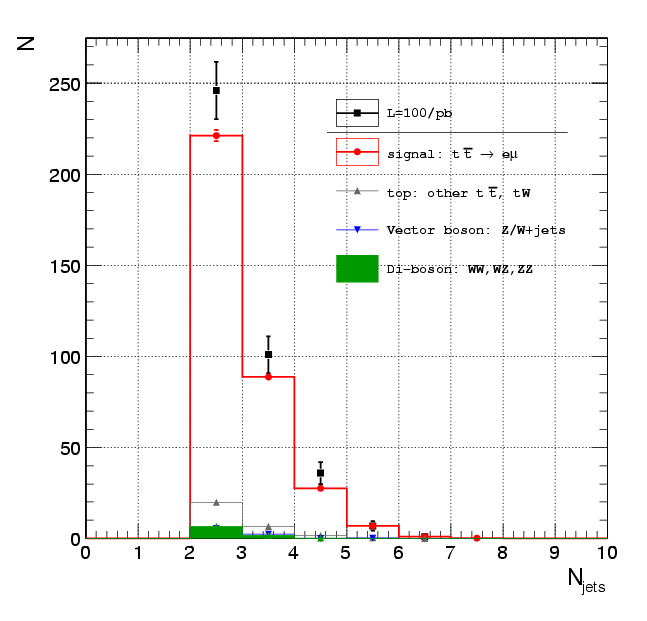
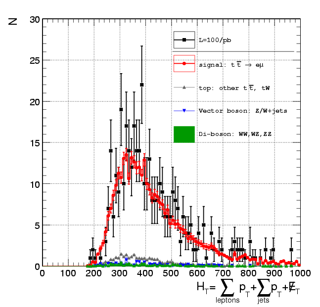
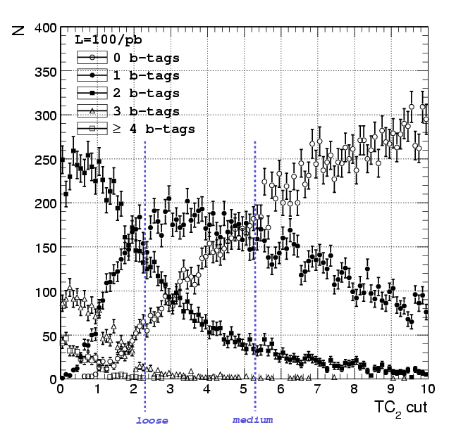
Control distributions
Below we show some control distributions for the selected events, that can be used for the dilepton channel.
| Jet multiplicity |
 |
 |
 |
 |
b-tag multiplicity (TC2) |
 |
 |
Background estimation from data
Flipped (and swapped)  method (summary)
Below we explore how to use a based method to subtract background from the data. The baseline idea is to build measure that, by a change variables, leaves the background invariant but not the signal. Having a with such probabilities one can do the following event selection:
- normal selection:
 - will select signal-like events with some quality criteria and some background events
- flipped selection:
 - will reject signal-like events but will select combinatorial background events
The is well constructed if both selections yields more or less the same background events leaving the distributions of interest (kinematics, b-tagging multiplicity, etc.) invariant.
By the procedure described above one obtains two distinct distributions  and
and  depending on the event selection used. By taking the difference of these distributions the background contributions will be eliminated effectively if the requirement for the is met. Then
  is equivalent to
  obtained from a 100% pure signal sample.
Next we discuss the construction of the having in mind these requirmentes.
obtained from a 100% pure signal sample.
Next we discuss the construction of the having in mind these requirmentes.
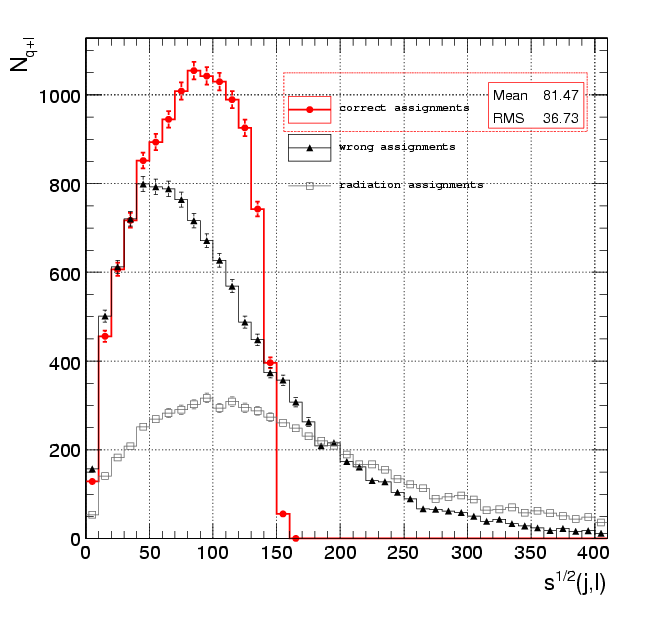
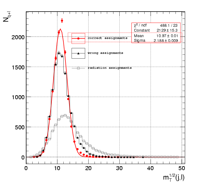
Jet + lepton kinematics based
As point of departure we choose 2 distributions based on the kinematics of the jet and lepton produced at a top decay vertex: the invariant mass and the transverse mass of the pair. The distributions, for these quantities, obtained at Monte-Carlo level, are shown below:
| Jet+lepton pair kinematics at Monte-Carlo level |
| Invariant mass |
Transverse mass (square root) |
 |
 |
 |
 |
For each event selected we proceed as follows:
- select the 2 highest leptons as the leptons from W decay generated after the top decay;
- if the number of selected jets is higher than 2 than we select the 3 jets with highest combined likelihood ratio value;
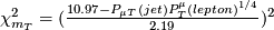
- try all jet+lepton combinations to build the matrix using the formulas from the table above;
- find the 2 jet+lepton pairs (excluding double-counting) that minimize the matrix;
- repeat the computation of the matrix but flipping the lepton's momentum -
 ;
;
We compute then the following quantities for the 2 pairs that minimize the matrix:
-
 - sum;
-
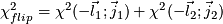 - inverting the 3-momentum of the leptons;
-
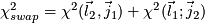 - swapping the leptons in each pair;
The table below shows the distributions obtained for signal and background events for these quantities:
| distributions |
| Event type |
Kinematics used in jet+lepton pairing |
| Invariant mass |
Transverse mass (square root) |
| Signal |
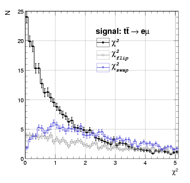 |
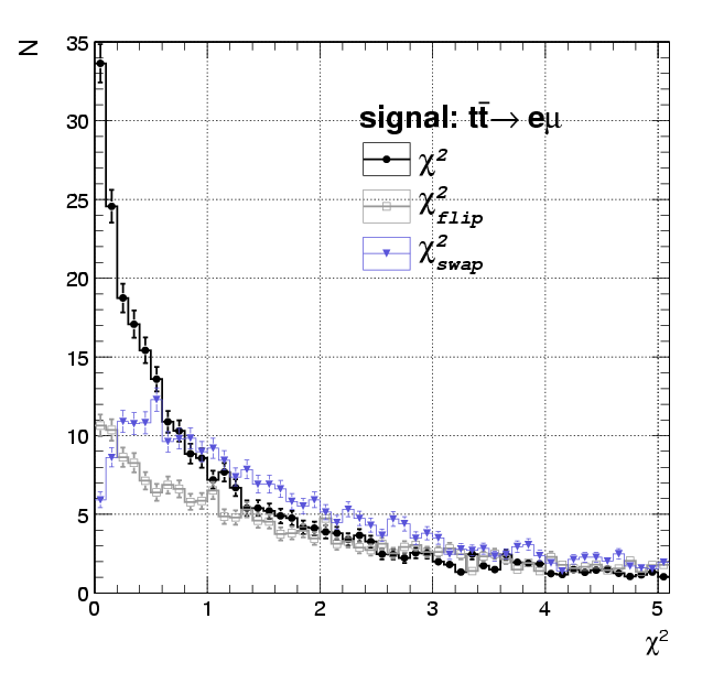 |
| Background |
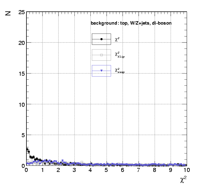 |
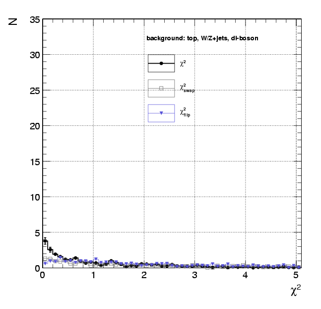 |
The coice of the cut  for is made maximizing the event yield after subtraction, that is, finding
  . The table below summarizes the cuts chosen for .
| Selection cut for distributions |
| Subtraction mode |
Kinematics used in jet+lepton pairing |
| Invariant mass |
Transverse mass (square root) |
| Flip |
3.35 |
2.45 |
| Swap |
2.15 |
0.75 |
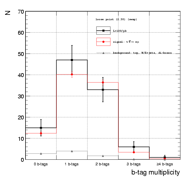
We select each event using the 3 defined above and the cuts defined in the previous table. For each selected event we compute the b-tag multiplicity for different values of the b-tagging discriminator. The distributions obtained for each selection are shown below. We also show the results obtained after subtracting the distribution obtained with the or  selections from the one obtained with the selection.
| b-tag multiplicity distributions |
| b-tag working point |
Full data |
After background subtraction |
| Invariant mass flip |
Invariant mass swap |
Transverse mass (square root) flip |
Transverse mass (square root) swap |
| Loose point for track counting (TC2=2.3) |
 |
 |
 |
 |
 |
| Medium point for track counting (TC2=5.3) |
 |
 |
 |
 |
 |
Latex rendering error!! dvi file was not created.
 Main Web>TWikiUsers>PedroSilva>PedroVtbMeasurementStudies>VtbDileptonicEventSelection (2008-11-19, PedroSilva)
 EditAttachPDF


