CMS Tutorial @ PKU -- From Zero to Expert
Upsilon Analysis Exercises
ZhenHu, FangzhouZhang, Sijin Qian Goal of this twiki This Twiki page presents a tutorial prepared for new CMS students at Peking University. We assume the attendees to be familiar with basic C++ and ROOT. Acknowledgments CMS Group at Purdue University, Fermilab LPC, EJTermContents:
Introduction
In these Exercises we will measure the Upsilon resonance cross section . The differential cross section is given by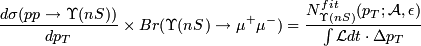
- acceptance A (see Exercise 2),
- efficiency ε (see Exercise 3),
- fitted yield N (see Exercise 4),
- and luminosity L.
Analysis Steps
Exercise 1 - Setup the working area
Release & Software
Log to a computing node (Currently we have node02~node15):ssh node02Create working directory, set cmssw release:
cp /md3000/scratch01/sw/cmsset_default.sh ./
source cmsset_default.sh

mkdir UpsilonAna
cd UpsilonAna
scramv1 list | grep CMSSW
cmsrel CMSSW_3_1_3

cd CMSSW_3_1_3/src
cmsenv
Set up CVS
export CVS_RSH=/usr/bin/ssh
export CVSROOT=:pserver:anonymous@cmscvs.cern.ch:/cvs_server/repositories/CMSSW
cvs login
The password is the famous CMS common password: 98passwd If you see an error message like
Unknown host cmscvs.cern.ch on some nodes, please change to another node. You'll need to use CVS to check out code and configuration files to your area so that you can modify and use them. ( Notice The frequently-used CVS package for Jpsi and Upsilon analysis is the official Onia2MuMucvs co -d zhenhu/PKUTutorial UserCode/zhenhu/PKUTutorial addpkg MuonAnalysis/MuonAssociators V01-01-00 addpkg PhysicsTools/TagAndProbe V01-08-01 addpkg MuonAnalysis/TagAndProbe V06-02-01 addpkg CondCore/PhysicsToolsPlugins V00-00-03-01 addpkg CondFormats/BTauObjects V01-03-00 addpkg CondFormats/DataRecord V06-07-03-01 addpkg CondFormats/PhysicsToolsObjects V01-02-07-01 addpkg RecoBTag/PerformanceDB V00-01-00 addpkg RecoBTag/Records V00-01-00 addpkg RecoMuon/Records V00-01-03 cd PhysicsTools/TagAndProbe patch -p0 < ../../zhenhu/PKUTutorial/test/tnp-v010801-p5.patch cd ../.. addpkg GeneratorInterface/Pythia6Interface V01-04-39 cd GeneratorInterface/Pythia6Interface patch -p0 < ../../zhenhu/PKUTutorial/test/pythia6PtGun_Rapidity.patch cd ../../PhysicsTools/TagAndProbe patch -p0 < ../../zhenhu/PKUTutorial/test/tripleGaussianLineShape.patch cd ../.. scramv1 b -j4
this takes a few minutes
Consider the test directory as the default working location
cd zhenhu/PKUTutorial/test
Exercise 2 - Calculation of Acceptance
The CMS detector does not cover the whole eta range therefore a fraction of Upsilons decaying to muons will not be detected. Also tracks from muons with low pT will not be identified as muons as the low pT muons cannot reach the muon system. Therefore there is a need to estimate what fraction of Upsilons can be detected assuming 100% detector efficiency. This fraction is called geometric and kinematic acceptance. In this analysis we accept muons in the pseudorapidity range |η| < 2.1. We make this choice to match the eta range of the single muon trigger. Within this range we assume full detector coverage. We also require both muons to have pT > 3.5 GeV to have sufficient muon identification and triggering efficiencies. The acceptance is a function of Upsilon pT, rapidity and polarization. To estimate the acceptance of Upsilons we rely on Monte Carlo simulations. In contrast, the efficiencies of muon identification and triggering can be estimated from the data with the Tag and Probe method, described below in Exercise 3. However, the efficiency of a muon being reconstructed with a track in the silicon tracking system needs MC simulations and therefore it is combined with the acceptance. Thus, out final definition of acceptance is the fraction of generated Upsilons decaying to muons that are reconstructed with silicon tracks of opposite charge with pT > 3.5 GeV and |η| < 2.1 and also the invariant mass is in the mass window of the Upsilon. Formally: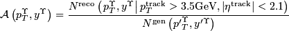
Step 1 - Generate an "Upsilon Gun" Data Sample
When generating Upsilon events with PYTHIA, the pT spectrum of Upsilons is steeply falling and the statistics of events at high pT is low. In addition, the presence of the underlying event prolongs the simulation of events significantly. Hence we use an "Upsilon gun" that produces events that contain only the Upsilon, distributed flat in pT and Rapidity, and the daughter muons with zero polarization. Then all events are full-simulated and reconstructed. TheupsilonGun_cfg.py job configuration in the test directory does the above mentioned steps. (For another generator examples, please see Upsilon1SupsilonGun_cfg.py contains the parameters of the "Pythia6PtGun" module:
process.generator = cms.EDProducer("Pythia6PtGun",
    PGunParameters = cms.PSet(
        MinPhi = cms.double(-3.14159265359),
        MinPt = cms.double(0.0),
        ParticleID = cms.vint32(553),
        MaxRapidity = cms.double(2.0),
        MaxPhi = cms.double(3.14159265359),
        MinRapidity = cms.double(-2.0),
        AddAntiParticle = cms.bool(False),
        MaxPt = cms.double(20.0)
    ),
...
The ID of Upsilon(1S) is 553. We are planning to measure the Upsilon cross section in the Rapidity range (-2,2) and pT range (0,20) GeV. Adjust the kinematic phase-space of the Upsilon to somewhat larger range as due to resolution effects an Upsilon generated outside the measured range can be reconstructed within. Please ensure that the Upsilons decay only to muons by changing the branching fraction as shown below:
pythiaUpsilonDecays = cms.vstring(
    'MDME(1034,1)= 0 ! 0.025200    ! e- e+',
    'MDME(1035,1)= 1 ! 0.024800    ! mu- mu+',
    'MDME(1036,1)= 0 ! 0.026700    ! tau- tau+',
    'MDME(1037,1)= 0 ! 0.015000    ! d dbar',
    'MDME(1038,1)= 0 ! 0.045000    ! u ubar',
    'MDME(1039,1)= 0 ! 0.015000    ! s sbar',
    'MDME(1040,1)= 0 ! 0.045000    ! c cbar',
    'MDME(1041,1)= 0 ! 0.774300    ! g g g',
    'MDME(1042,1)= 0 ! 0.029000    ! gamma g'),
The schedule clearly shows the executed steps: generation, simulation,...,reconstruction:
process.schedule = cms.Schedule(
  process.generation_step,
  process.simulation_step,
  process.digitisation_step,process.L1simulation_step,process.digi2raw_step,process.raw2digi_step,
  process.reconstruction_step)
It would require significant space to save every object in the output file. Therefore, to save space, an analyzer has been prepared
DimuonTree.cc in the ../src directory that dumps only the necessary variables into a TTree.
This basic code will also allow you to understand how to access information from a data sample root file. Fifteen parameters are saved into a TTree, including the generated momenta of Upsilons and muons along with the momenta of reconstructed tracks.
Adjust the number of required events to 100 events:
process.maxEvents = cms.untracked.PSet(
    input = cms.untracked.int32(100)
)
Test the configuration by running
cmsRun upsilonGun_cfg.pyTo check the output, open the resulting upsilonGun.root file:
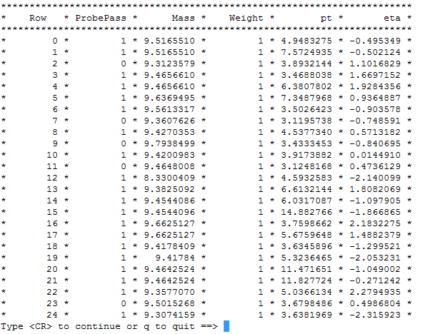
root -l upsilonGun.root
root [1] TBrowser b
Click on "ROOT Files", and then "upsilonGun.root" and then "UpsTree", you will find 15 branches inside. Click on each branch, to see the distribution of each parameter. Or you can scan the contents of the tree:
root [2] UpsTree->Scan("*");
It will display all the branches in the tree like below:
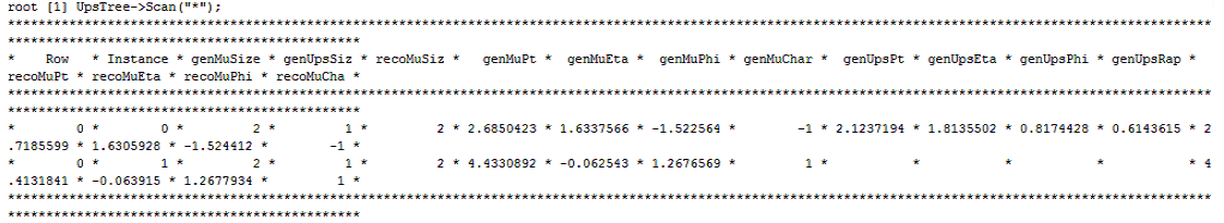
Notice: The generated values of the Y and muons depends on the random number generator in Pythia and so differ from the above example. However, the structure of the tree is the same.
If everything looks fine, please log on the CERN computing server (lxplus.cern.ch), or log on our T3 site at Peking University (grid08.phy.pku.edu.cn). Then you can submit a CRAB job to produce larger statistics.
Notice: You have to create the same CMSSW working area before submitting CRAB jobs.


Modify the
upsilonGun_cfg.crab configuration to submit 100 jobs producing 500 events each.
First initiate your proxy:
voms-proxy-init -voms cmsSet up CRAB:
source /home/cmssoft/CRAB/CRAB_2_6_6/crab.shThen execute:
crab -create -submit -cfg upsilonGun.crabTo check the job status, run:
crab -status -c upsilonGunEach event takes about 2 seconds, so the jobs will run for about 20 minutes. In the meantime one could start working on Step 2. When all jobs are "Done", retrieve the output with
crab -getoutput -c upsilonGun
upsilonGun/res/ directory. To merge them, use the standard ROOT tool
hadd -f upsilonGun.root upsilonGun/res/upsilonGun_*.rootThe resulting data sample is saved in upsilonGun.root (overwriting the previous version).
Step 2 - Calculate Acceptance
Since the acceptance depends on the pT and Rapidity of the Upsilon, we calculate it in bins of pT and Rapidity. The polarization dependence will be studied as a systematic uncertainty. We are still in the directory "zhenhu/PKUTutorial/test". There is a ROOT macro named "acceptance.C". It defines a two dimensional histogram for the generated Upsilon pT and Rapidity and it is filled for each event of the upsilonGun.root sample generated in the previous exercise.
TH2F* genPtRap = new TH2F("genUps","",4,0,20,4,-2,2);
for(int i=0; i < t->GetEntries(); i++){
  genPtRap->Fill( genUpsPt[0], genUpsRapidity[0] );
  ...
}
There is another 2D histogram, which is a copy of the above, that collects events in which the Upsilon is reconstructed with two tracks of opposite charge, pT > 3.5 GeV, |η| < 2.1 and invariant mass within 1.0 GeV of the PDG value 9.46 GeV.
TH2F* recoPtRap = (TH2F*)genPtRap->Clone("recoUps");
for(int i=0; i < t->GetEntries(); i++){
  if ( recoMuCharge[tr1]*recoMuCharge[tr2] == -1 && recoMuPt[tr1] >= 3.5 && recoMuPt[tr2] >= 3.5 && fabs(recoMuEta[tr1]) < 2.1 && fabs(recoMuEta[tr2]) < 2.1 ){
    ...
    if( minDeltaM < 1.0 ){
      recoPtRap->Fill( recoUpsPt, recoUpsRapidity );
    }
  }
}
The ratio of the two histograms is the acceptance by definition.
acc->Divide(recoPtRap, genPtRap, 1, 1, "B");To run the macro:
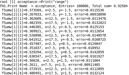
make acceptance #compiles acceptance.C
./acceptance upsilonGun.root acceptance.root
To print out the result:
root -l acceptance.root
root [1] acceptance->Print("range")
grid09.phy.pku.edu.cn). You can transfer it to your local directory and give it a new name upsilonGun_new.root:
scp PKUTutorial@grid09.phy.pku.edu.cn:/md1000_1/user/zhenhu/Tutorial/upsilonGun.root ./upsilonGun_new.rootThe passwd for the user PKUTutorial is 111111.
Notice: If you can not use the scp transfer, try to logout the node you are working on, and then log in hepfarm01 or hepfarm02.
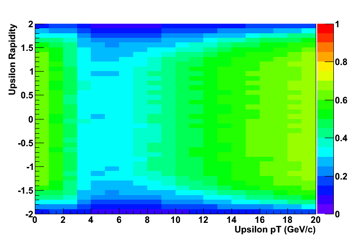
Now the binning of the acceptance can be refined. Please adjust it to pT (20,0,20) and Rapidity (40,-2,2) in the acceptance.C and run:
make acceptance
./acceptance upsilonGun_new.root acceptance.root
The result can be plotted with
acceptancePlot.C that saves an acceptance.png figure.
root -b -q acceptancePlot.C
Quiz1: Please write a piece of C++ code to plot the muon pT distribution, muon eta distribution, Upsilon pT distribution, and Upsilon eta distribution at generator level.
Quiz2: Please write a piece of C++ code to plot the muon pT distribution, muon eta distribution, Upsilon pT distribution, and Upsilon eta distribution at reconstruction level.
Quiz3: In what pT range can the Upsilon cross section be measured if we accept muons only with pT > 10 GeV?
Exercise 3 - Using Tag and Probe to measure efficiencies
Tag and Probe methodology Tag and Probe (T&P) is a data driven method for efficiency calculations. It utilizes resonances to identify probe objects. Assuming no efficiency correlation between the two decay products of the resonance it identifies one of the muons, called a Tag, using tight identification criteria and measures the efficiency of the other muon, referred to as a Probe. For detailed explanation of Tag and Probe analysis of Upsilon, please readCMS AN2009_119.
Efficiency components: - Tracking efficiency (assuming it to be 1)
- Tracker muon ID efficiency
- Trigger efficiency
Step 1 - Skim the Data Samples
A MC data sample equivalent to 1.87/pb integrated luminosity (455492 events) has been produced to use in the exercise, and is located atgrid09.phy.pku.edu.cn:/md1000_1/user/zhenhu/Tutorial/skim_1.87pb-1.root . Please scp transfer it to your working directory.
Next it's explained how this was put together, starting from officially produced samples.
- List of signal and background central monte carlo datasets on DBS
-
/Upsilon1S/Summer09-MC_31X_V3_7TeV-v1/GEN-SIM-RECO -
/Upsilon2S/Summer09-MC_31X_V3_7TeV-v1/GEN-SIM-RECO -
/Upsilon3S/Summer09-MC_31X_V3_7TeV-v1/GEN-SIM-RECO -
/ppMuMuX/Summer09-MC_31X_V3_7TeV-v1/GEN-SIM-RECO
-
Go to the DBS webpage, search the dataset "/Upsilon1S/Summer09-MC_31X_V3_7TeV-v1/GEN-SIM-RECO ". First make a note of the total number of events in this dataset: "contains 1166738 events". Then click on its parents, then click Conf.files. You can see the configuration file used for generating Upsilon1S to dimuon samples. Inspect the contents and notice the lines below:
Submit CRAB jobs since the dataset is not located at PKU.
Inspect the CRAB configuration file test/skimUpsilon.crab . To submit the job:
". First make a note of the total number of events in this dataset: "contains 1166738 events". Then click on its parents, then click Conf.files. You can see the configuration file used for generating Upsilon1S to dimuon samples. Inspect the contents and notice the lines below:
Submit CRAB jobs since the dataset is not located at PKU.
Inspect the CRAB configuration file test/skimUpsilon.crab . To submit the job:
filterEfficiency = cms.untracked.double(0.139),
The "filterEfficiency" has to do with the filter that is used in the generation (like cuts on muon Pt and Eta). It is defined as the ratio between events passing the filter and the total number of generated events by PYTHIA. For example if the filterEfficiency is 0.01, it means of every 100 events PYTHIA generates, only 1 events is of interest for us, and 99 events are thrown away.
comEnergy = cms.double(7000.0),
The center-of-mass energy is 7 TeV.
crossSection = cms.untracked.double(99900.0),
The number in "crossSection" is a value in [pb] and is the product of two factors:
1) The production cross-section "sigma" with which the particle is produced.
2) The forced branching ratio, "BR", leading to the desired decay mode in which the particle should be looked for:
'MDME(1035,1)=1 ! 0.024800 mu- mu+',The integrated luminosity is the number of events before filter divided by the production cross-section. In this case, it should be (1166738/0.139)/99900 = 84.02 /pb . Similarly, we calculated the intergrated luminosity of the other datasets. And we see the background sample "ppMuMuX" has the smallest integrated luminosity 1.87/pb. So to make things more realistic, we decide to use 1.87/pb signal samples to make the level of signal and background compatible. To do this, we just need to calcuate how many events we need for the signals. Take Upsilon 1S for example again. We already measured the integrated luminosity of Upsilon 1S dataset is 84.02/pb corresponding to 11667380 events. So for 1.87/pb, we should have 1166738*(1.87/84.02) = 25967 events. For Upsilon 2S and 3S, we just repeated this calculation. Skim the Data Samples Inspect the python configuration file: skimUpsilon_cfg.py
crab -create -submit -cfg skimUpsilon1S_7TeV.crab
crab -status -c skimUpsilon1S_7TeV
When the jobs are done:
crab -getoutput -c skimUpsilon1S_7TeV
cd skimUpsilon1S_7TeV/res
merge_cfg.py in order to make a date-like soup. As it will take a while to produce them, we have prepared it as pointed to above.
Step 2 - Produce tag-and-probe Ntuples
We will use tracker muons in this analysis. First, we need to select the good tracker muons that satisfy the offline selection cuts (with good track quality in geometric and kinematic acceptance). We prepared this file "MuonSelectorUpsilon.cc" to select good tracker muons. Please move this module code:cp ../src/MuonSelectorUpsilon.cc ../../../MuonAnalysis/TagAndProbe/plugins/Open the file
MuonSelectorUpsilon.cc
vi ../../../MuonAnalysis/TagAndProbe/plugins/MuonSelectorUpsilon.ccUncomment the last three lines in the file to make it as a CMSSW Plugin now:
/*
/// Register this as a CMSSW Plugin
#include "FWCore/Framework/interface/MakerMacros.h"
DEFINE_FWK_MODULE(MuonSelectorUpsilon);
*/
Then compile:
cd ../../..
scramv1 b
Make sure you are still in the
/test directory. We prepared this configuration file "tnp_from_skim.py" to produce the Tag and Probe Ntuple.
cmsRun tnp_from_skim.py
it will take ~40 minutes to finish. There are about 470000 events in total.
Two root files will be produced. (For your convenience, a backup of these two files are also stored in grid09.phy.pku.edu.cn:/md1000_1/user/zhenhu/Tutorial/). Each of them will contain a TTree, with invariant mass, pt, eta and passing/failing information for measuring tracker muon ID or trigger efficiency -
histo_output_MuFromTkUpsTkM.rootis for the tracker muon identification efficiency -
histo_output_HltFromUpsTkM.rootis for the trigger efficiency
root -l histo_output_MuFromTkUpsTkM.root
root [1] fitter_tree->Scan("");
Step 3 - Compute the efficiences
We supposed that you are still in /test . Start fitting:cmsRun fit_tnp_Id_cfg.py cmsRun fit_tnp_trigger_cfg.py
This part will take ~15min to finish
Once the jobs finish, there will be a root file containing fitting results produced for each tag and probe Ntuple:
process.fitMuFromTkUpsTkM = RunFit.clone(
    ReadFromFiles = [ 'histo_output_MuFromTkUpsTkM.root' ],
    FitFileName   =     'fit_result_MuFromTkUpsTkM.root'  ,
)
process.fitHltFromJPsiTkM = RunFit.clone(
    ReadFromFiles = [ 'histo_output_HltFromUpsTkM.root' ],
    FitFileName   =     'fit_result_HltFromUpsTkM.root'  ,
    Var2BinBoundaries   = cms.untracked.vdouble( -2.1,-1.2,0.0,1.2,2.1),
)
Each fit_result file contains fitting plots in each pt/eta bin along with efficiencies via Tag and Probe or MC truth.
For example:
root -l fit_result_MuFromTkUpsTkM.root
root [1] TBrowser b
Click on the root file name:
root [2] fit_canvas_pt_1_eta_1->Draw(" ");
You will see the mass fitting plots of "all probes", "passing probes", "failing probes" for tracker muon ID efficiency in pt (4.5, 6), eta (-1.2,0):

root [3] gStyle->SetPalette(1);
root [4] gStyle->SetOptStat(0);
root [5] fit_eff_pt_eta->Draw("colz");
root [6] fit_eff_pt_eta->DrawCopy("text same");
root [7] fit_canvas_pt_1_eta_1->SetLogx();
root [8] fit_eff_pt_eta->GetXaxis()->SetMoreLogLabels();
The tracker muon ID efficiency from Tag and Probe in each eta and pt bin is displayed:

Eventually, Tag and Probe method will be performed on real data to get efficiencies. In Monte Carlos data samples, we don't have any trigger bias in them. That is to say, we have both the events which pass trigger and the events which are not be able to pass trigger. And we are able to know whether an event passing trigger or not. However, in real data, the events will pass trigger first and then come to us. Therefore, we always have a subset of all the events. Then the question is, will the trigger efficiency measured from real data (with trigger bias) be consistent with the one measured from Monte Carlos data samples (without trigger bias)? Let's do this studies step by step as below.
1) Produce data samples with trigger bias
We don't want to waste time to make the skimmed soup again. Instead, we will change the configuration file "tnp_from_skim.py" to force Tag and Probe only performed on those events which pass trigger.
Add the following lines in the "tnp_from_skim.py" just after the definition of "PASS_HLT":
process.triggerMuons = cms.EDFilter("PATMuonRefSelector",
    src = cms.InputTag("patMuons"),
    cut = cms.string( PASS_HLT ),
    filter = cms.bool(True),
)
This filter simply filters events by checking whether the event contains at least one pat muon which can pass the "HLT_Mu3" trigger path. If the size of the so-called "triggerMuons" is not zero, then this event must pass the "HLT_Mu3" trigger. Otherwise, it must not. Only the events passing "HLT_Mu3" will be keeped after this filter.
Don't forget to add this process beyond all of the other processes.
2) Repeat Exercise 3 with the new "tnp_from_skim.py". Notice, when fitting the histograms, you only need to run the "fit_tnp_trigger_cfg.py" because only the trigger efficiencies may be affected due to the trigger bias. Also, please save the output files into different names. You can add "_bias" as an extension of each file name.
QUIZ: Are these differences between the tag and probe efficiencies measured from non-bias samples and bias samples?
If the answer to the above quiz is "yes", please continue doing the next step.
3) Open the "tnp_from_skim.py" again and check the tagMuons requirements:
process.tagMuons = cms.EDFilter("PATMuonRefSelector",
    src = cms.InputTag("patMuons"),
    cut = cms.string("isGlobalMuon && pt > 3 && abs(eta) < 2.4 "),
    filter = cms.bool(True),
)
QUIZ: Modify the above lines to require tag muons passing trigger.
Once you've done the quiz, repeat 2) with the new "tnp_from_skim.py". Save output files into new names.
QUIZ: Compare the efficiencies measured from 3) to the previous two tset of trigger efficienies. What will you conclude?
Exercise 4 - Upsilon Selection and Yield Tree
The purpose of this exercise is to create a ROOT TTree with the Upsilon candidate information to be used for fitting the signal yield. The input is the skimmed data sample that contains the PAT objects, produced in the previous exercise. The output TTree has to contain the mass, pt and rapidity of the Upsilon candidates, as well as the pt and eta of the daughter muons for efficiency corrections. Technically this task consist of two parts: A CMSSW python configuration upsilonYield_cfg.pyStep 1 - Produce the data tree from the skim
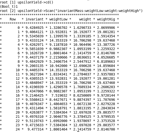
Change the Event number to -1 and run the prepared configuration:cmsRun upsilonYield_cfg.pyInspect the output root file:
root -l upsilonYield.root
root [1] upsilonYield->cd()
root [2] upsilonYield->Scan()

Step 2 - Apply selection
QUIZ: Modify test/upsilonYield_cfg.py to select muons with additional quality cuts:- number of valid silicon hits > 10
- normalized chi2 of silicon fit < 5
- TMOneStationTight tracker muon selection
upsilonYield_cfg.py should contain the following:
process.goodMuonsOld = cms.EDFilter("PATMuonRefSelector",
    src = cms.InputTag("patMuons"),
    cut = cms.string("track.isNonnull && pt > 3.5 && abs(eta) < 2.1"),
)
process.goodMuons = cms.EDProducer("MuonSelectorUpsilon",
    src = cms.InputTag("goodMuonsOld"),
    selectGlobalMuons = cms.bool(False)
)
Rerun the job to obtain the new tree.
Exercise 5 - Cross Section
We have now the various ingredients in place for estimating the cross section.

- L denotes the luminosity of the sample.
- ΔpT is the width of the dimuon pT bin
- N is the corrected yield
Step 1 - Acceptance and efficiency corrections
In the first step, the event weights are computed, and appended to the data yield tree. The ROOT macro makeWeights.CupsilonYield.root , as well as the efficiency and acceptance files as input and produce an output file upsilonYieldWeighted.root that contains the same upsilonYield tree but with the weight column included in addition.
Please verify these files are available in the current working directory, or otherwise gather them there.
upsilonYield.root
acceptance.root
fit_result_MuFromTkUpsTkM.root
fit_result_HltFromUpsTm.root
To run it execute:
root -b -q 'makeWeights.C("upsilonYield.root", "acceptance.root", "fit_result_MuFromTkUpsTkM.root", "fit_result_HltFromUpsTm.root", "upsilonYieldWeighted.root")'
Step 2 - Fit the upsilon mass spectra
The baseline code for the cross section fitting part of the exercise is implemented in oniafitter.CbuildPdf, readData, fitYield .
Fitting is performed with the standard minuit/root/roofit tools. The program may be executed as follows.
root -l -b -q oniafitter.C >& log &or
root -l
root [0]  .L oniafitter.C+
root [0]  oniafitter()
You'll need to edit the code to select the various steps you like to be run. The model description for the signal and background mass distributions need to be specified. A simple model is provided, which assigns a second order polynomial pdf for the background, while the signal peaks are each described by a double gaussian (along with tail polynomial to account for final state radiation). Quiz: Inspect the provided pdf implementations
 RooAbsPdf  *pdf  = new RooAddPdf("pdf","total signal+background pdf",
				   RooArgList(*sigPdf,*bkgPdf),RooArgList(*nsig,*nbkg));
Start with the buildPdf method, and especially verify the signal and background functions.
un-comment code:
  /// fit raw yield
  fitYield(*ws,"total");
  plotMass(figs_ + "/mass_raw.gif",*ws);
Step 3 - Extract the corrected yield
The efficiency and acceptance corrections are embedded in the event weights, which were computed and added to the input root three previously. The corrected yield is extracted by repeating the fit to the weighted dataset. Quiz: Run the weighted fit over the full sample.
un-comment code:
 /// fit corrected yield
  ((RooDataSet*)ws->data("data"))->setWeightVar(*ws->var("weight"));
  fitYield(*ws,"total");
  plotMass(figs_ + "/mass_wei.gif",*ws);
Step 4 - Extract the cross section
Total, σ
All left to do is to retrieve the measured yields from the saved fit results, and normalize by the sample's luminosity (1.87 pb-1). Quiz: Compute the total cross section.
un-comment code:
 /// total cross section
  xsectTot(*ws);
Differential, dσ/dpT
For extracting the differential cross section, the dataset is divided in bins of dimuon transverse momentum (this quantity is part of the input root tree), and the fitting procedure used above is applied to the individual pT-bin sub-samples. Quiz: Compute the differential total cross section.
un-comment code:
 /// cross section vs pT
  xsectDif(*ws,true);
note: set argument to false if fits do not need to be repeated
Extract the yields from the individual peaks, and repeat the procedure above.
Your comments and feedback
-- ZhenHu - 13-Jan-2010

| I | Attachment | History | Action | Size | Date | Who | Comment |
|---|---|---|---|---|---|---|---|
| |
IdEffPtEta.png | r1 | manage | 52.3 K | 2010-01-14 - 12:56 | ZhenHu | |
| |
acceptance.png | r1 | manage | 7.3 K | 2010-01-14 - 12:55 | ZhenHu | |
| |
acceptance2.png | r1 | manage | 10.2 K | 2010-01-14 - 12:41 | ZhenHu | |
| |
acceptancePrint.png | r1 | manage | 21.3 K | 2010-01-14 - 12:55 | ZhenHu | |
| |
fitplot.png | r1 | manage | 64.7 K | 2010-01-14 - 12:56 | ZhenHu | |
| |
fitplot_3signal.jpg | r1 | manage | 72.9 K | 2010-01-14 - 12:56 | ZhenHu | |
| |
mass_raw.gif | r1 | manage | 9.0 K | 2010-01-14 - 12:57 | ZhenHu | |
| |
mass_wei.gif | r1 | manage | 9.7 K | 2010-01-14 - 12:57 | ZhenHu | |
| |
scan.png | r1 | manage | 79.0 K | 2010-01-14 - 12:58 | ZhenHu | |
| |
scanout.png | r1 | manage | 79.0 K | 2010-01-14 - 13:00 | ZhenHu | |
| |
tnptree.png | r1 | manage | 26.1 K | 2010-01-14 - 13:01 | ZhenHu | |
| |
triggerEffPt.png | r1 | manage | 40.0 K | 2010-01-14 - 13:01 | ZhenHu | |
| |
upsilonYield.png | r1 | manage | 74.8 K | 2010-01-14 - 13:02 | ZhenHu | |
| |
upsilonYieldWeighted.png | r1 | manage | 37.5 K | 2010-01-14 - 13:03 | ZhenHu | |
| |
upsilonpt.png | r1 | manage | 13.5 K | 2010-01-14 - 13:02 | ZhenHu |
Webs
- ABATBEA
- ACPP
- ADCgroup
- AEGIS
- AfricaMap
- AgileInfrastructure
- ALICE
- AliceEbyE
- AliceSPD
- AliceSSD
- AliceTOF
- AliFemto
- ALPHA
- Altair
- ArdaGrid
- ASACUSA
- AthenaFCalTBAna
- Atlas
- AtlasLBNL
- AXIALPET
- CAE
- CALICE
- CDS
- CENF
- CERNSearch
- CLIC
- Cloud
- CloudServices
- CMS
- Controls
- CTA
- CvmFS
- DB
- DefaultWeb
- DESgroup
- DPHEP
- DM-LHC
- DSSGroup
- EGEE
- EgeePtf
- ELFms
- EMI
- ETICS
- FIOgroup
- FlukaTeam
- Frontier
- Gaudi
- GeneratorServices
- GuidesInfo
- HardwareLabs
- HCC
- HEPIX
- ILCBDSColl
- ILCTPC
- IMWG
- Inspire
- IPv6
- IT
- ItCommTeam
- ITCoord
- ITdeptTechForum
- ITDRP
- ITGT
- ITSDC
- LAr
- LCG
- LCGAAWorkbook
- Leade
- LHCAccess
- LHCAtHome
- LHCb
- LHCgas
- LHCONE
- LHCOPN
- LinuxSupport
- Main
- Medipix
- Messaging
- MPGD
- NA49
- NA61
- NA62
- NTOF
- Openlab
- PDBService
- Persistency
- PESgroup
- Plugins
- PSAccess
- PSBUpgrade
- R2Eproject
- RCTF
- RD42
- RFCond12
- RFLowLevel
- ROXIE
- Sandbox
- SocialActivities
- SPI
- SRMDev
- SSM
- Student
- SuperComputing
- Support
- SwfCatalogue
- TMVA
- TOTEM
- TWiki
- UNOSAT
- Virtualization
- VOBox
- WITCH
- XTCA
Welcome Guest Login or Register
 |
|
or Ideas, requests, problems regarding TWiki? use Discourse or Send feedback